── Attaching packages ─────────────────────────────────────── tidyverse 1.3.2 ──
✔ ggplot2 3.3.6      ✔ purrr   0.3.5
✔ tibble  3.1.8      ✔ dplyr   1.0.10
✔ tidyr   1.2.1      ✔ stringr 1.4.1
✔ readr   2.1.3      ✔ forcats 0.5.2
── Conflicts ────────────────────────────────────────── tidyverse_conflicts() ──
✖ dplyr::filter() masks stats::filter()
✖ dplyr::lag() masks stats::lag()10 scale()
10.1 公共参数
公共参数name,breaks,labels,limits
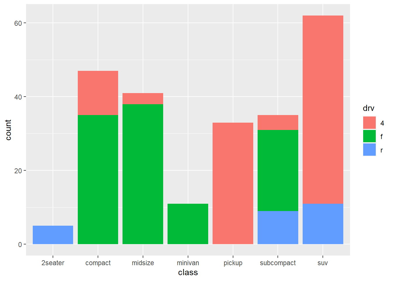
10.1.1 离散型 例 1

#更改图例名字 #
p0 + scale_fill_discrete(name="class") 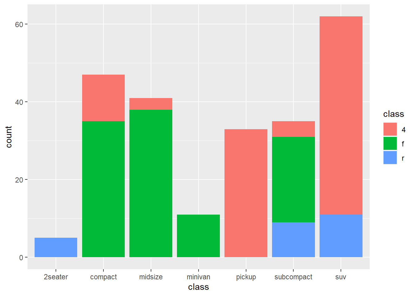
# 对应指定并更改图例标签 #
p0 + scale_fill_discrete (breaks = c("4", "r", "f"),
                          labels = c("four", "rr", "rr"))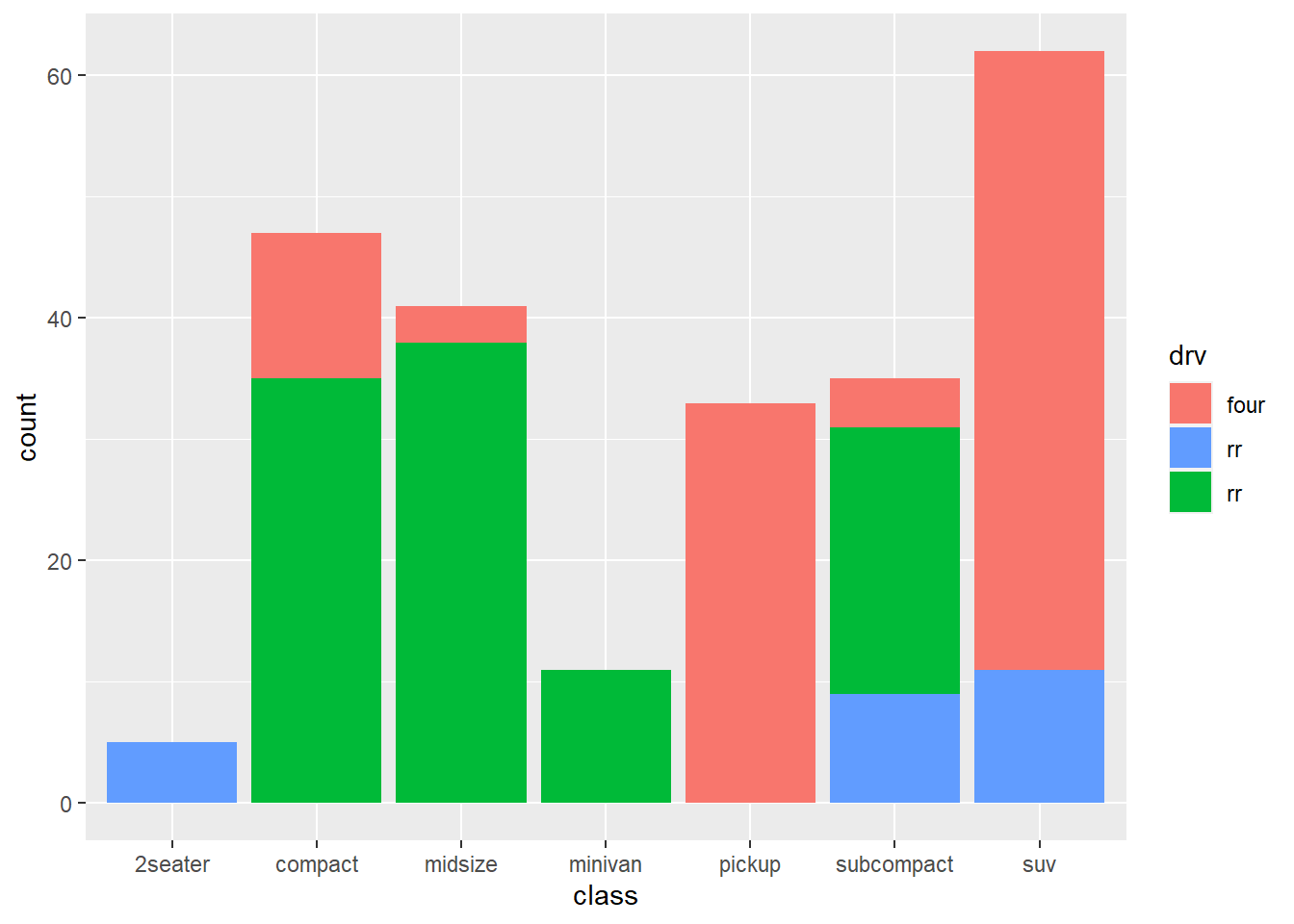
# 只显示4和r对应部分#
p0 + scale_fill_discrete (limits=c("4", "r")) 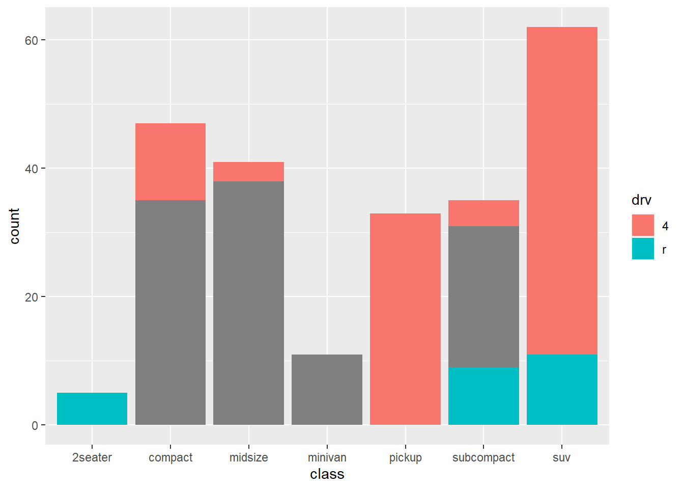
# 多出一个分类#
p0 + scale_fill_discrete (limits=c("4", "r", "f", "6"))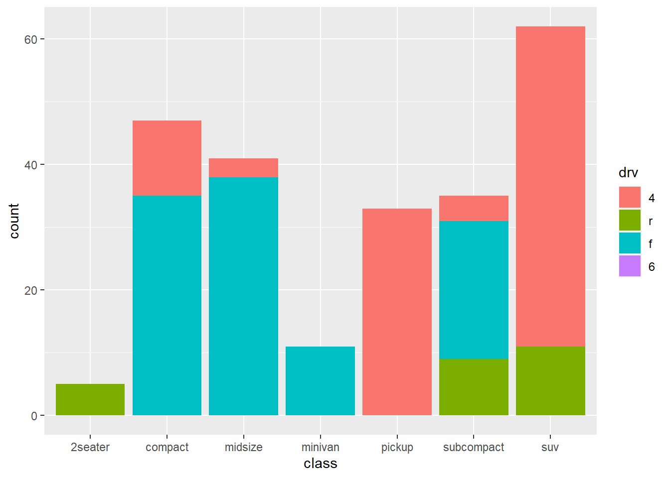
10.1.2 离散型 例 2
p1 <- ggplot(mtcars, aes(factor(cyl), mpg)) + geom_point();p1
p1 + scale_x_discrete(name="cyl") 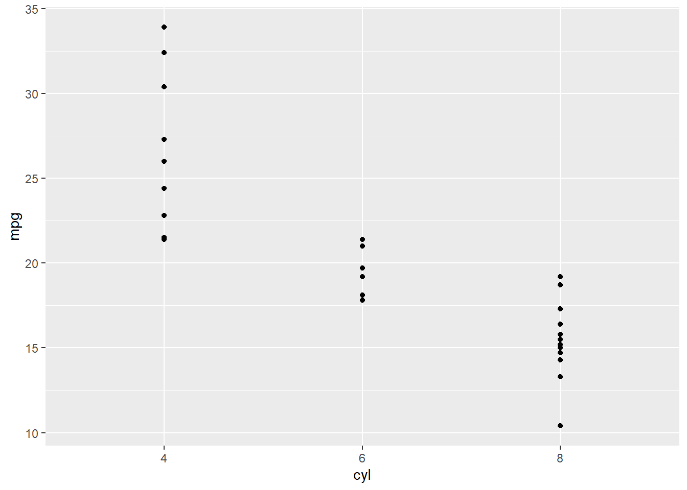
p1 + scale_x_discrete(labels = c("4"="a","6"="b","8"="c")) 
p1 + scale_x_discrete(labels = letters[1:3],breaks=c("4","6","8")) 
p1 + scale_x_discrete(labels = c("4"="a","6"="b"))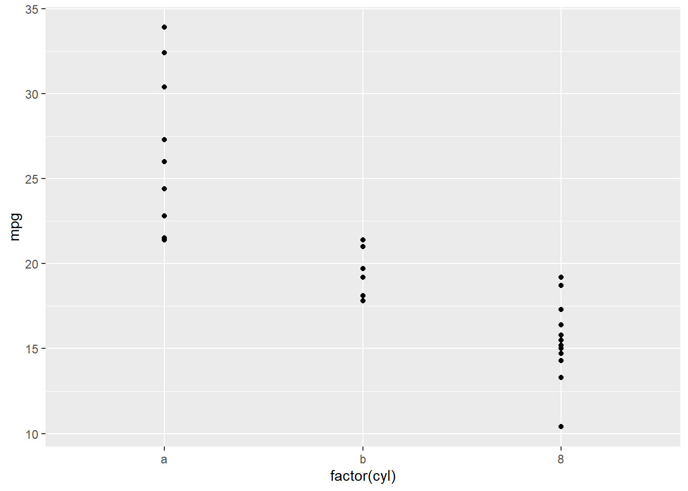
p1 + scale_x_discrete(labels = letters[1:3])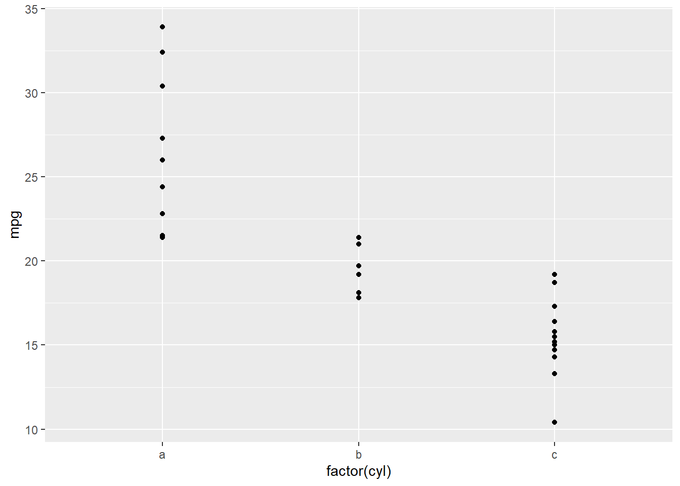
p1 + scale_x_discrete(limits=c("4","6"))Warning: Removed 14 rows containing missing values (geom_point).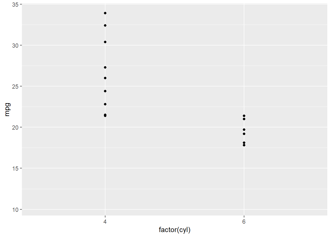
10.1.3 连续型 例 1
p2<-ggplot(mpg,aes(displ, hwy , color = cyl))+geom_point();p2
p2 +scale_color_continuous (name="Cyl",
                            breaks=c(7.5,6.2,4.9),
                            labels=c("a","b","c"))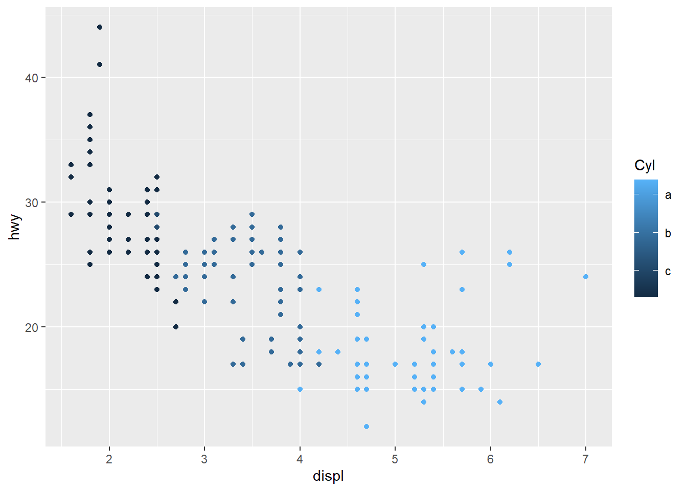
p2 +scale_color_continuous (name="CYL",
                            limits=c(5,6.8))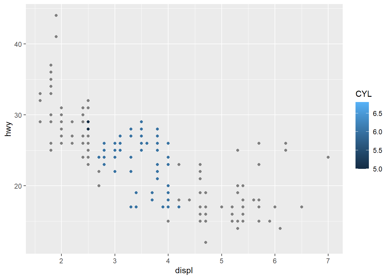
10.1.4 连续型 例 2
p3 <- ggplot(mtcars, aes(factor(cyl), mpg)) + geom_point();p3
p3 + scale_y_continuous("ylab_mpg")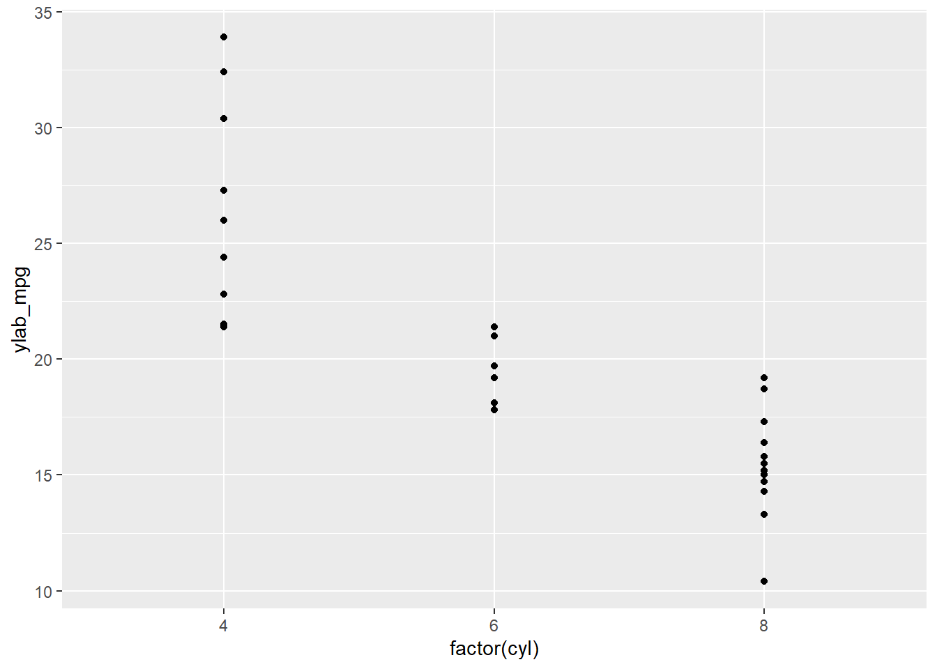
p3 + scale_y_continuous(breaks = c(10,20,30))
p3 + scale_y_continuous(breaks = c(10,20,30), labels=scales::dollar)
p3 + scale_y_continuous(limits = c(10,30))Warning: Removed 4 rows containing missing values (geom_point).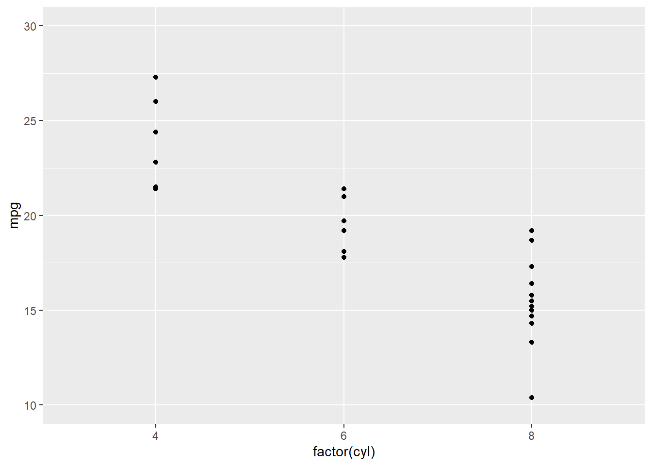
p3 + scale_y_reverse() # 纵坐标翻转,小数在上面,大数在下面#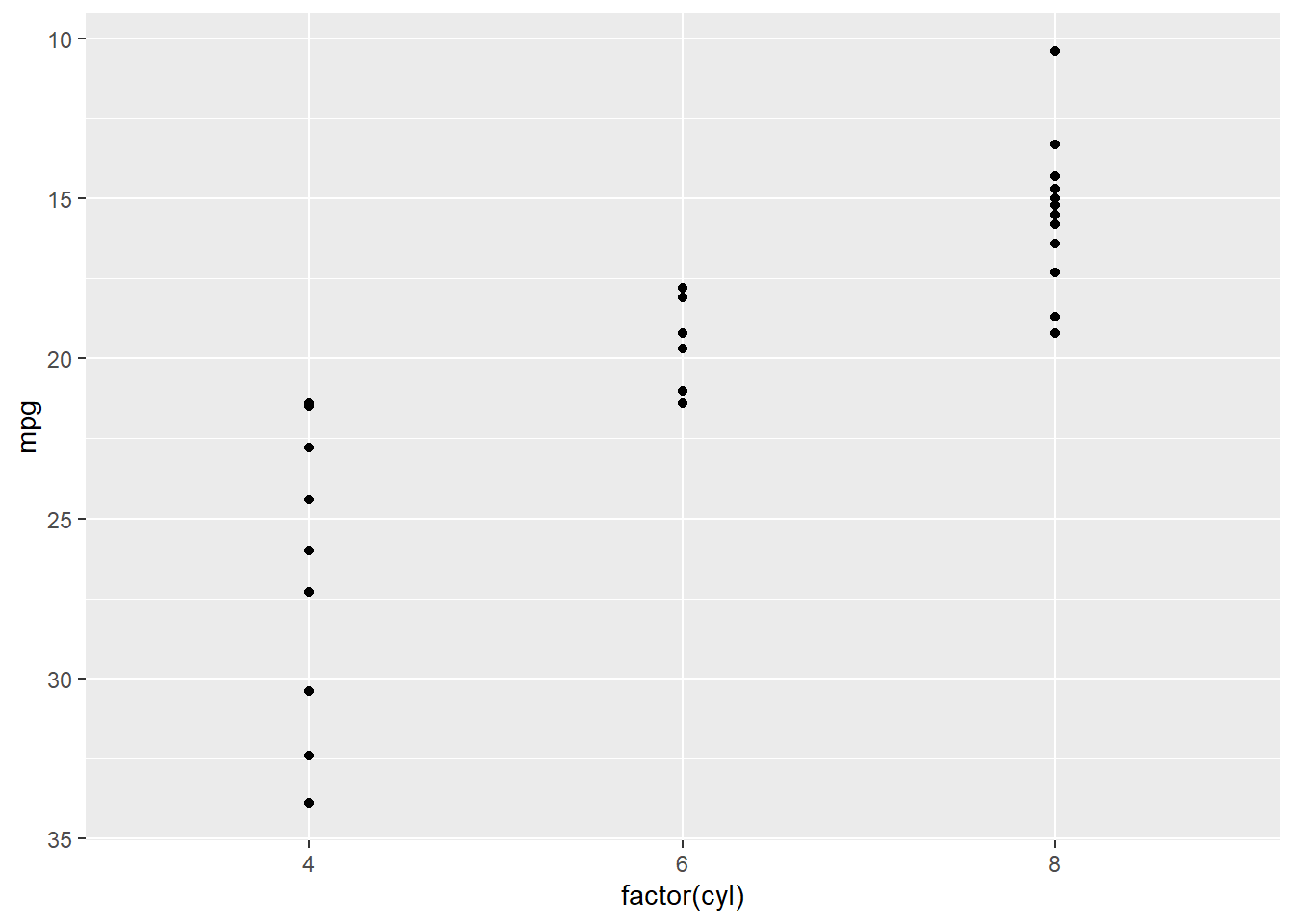
p3 + scale_y_log10()
p3 + scale_y_continuous(trans = "log10")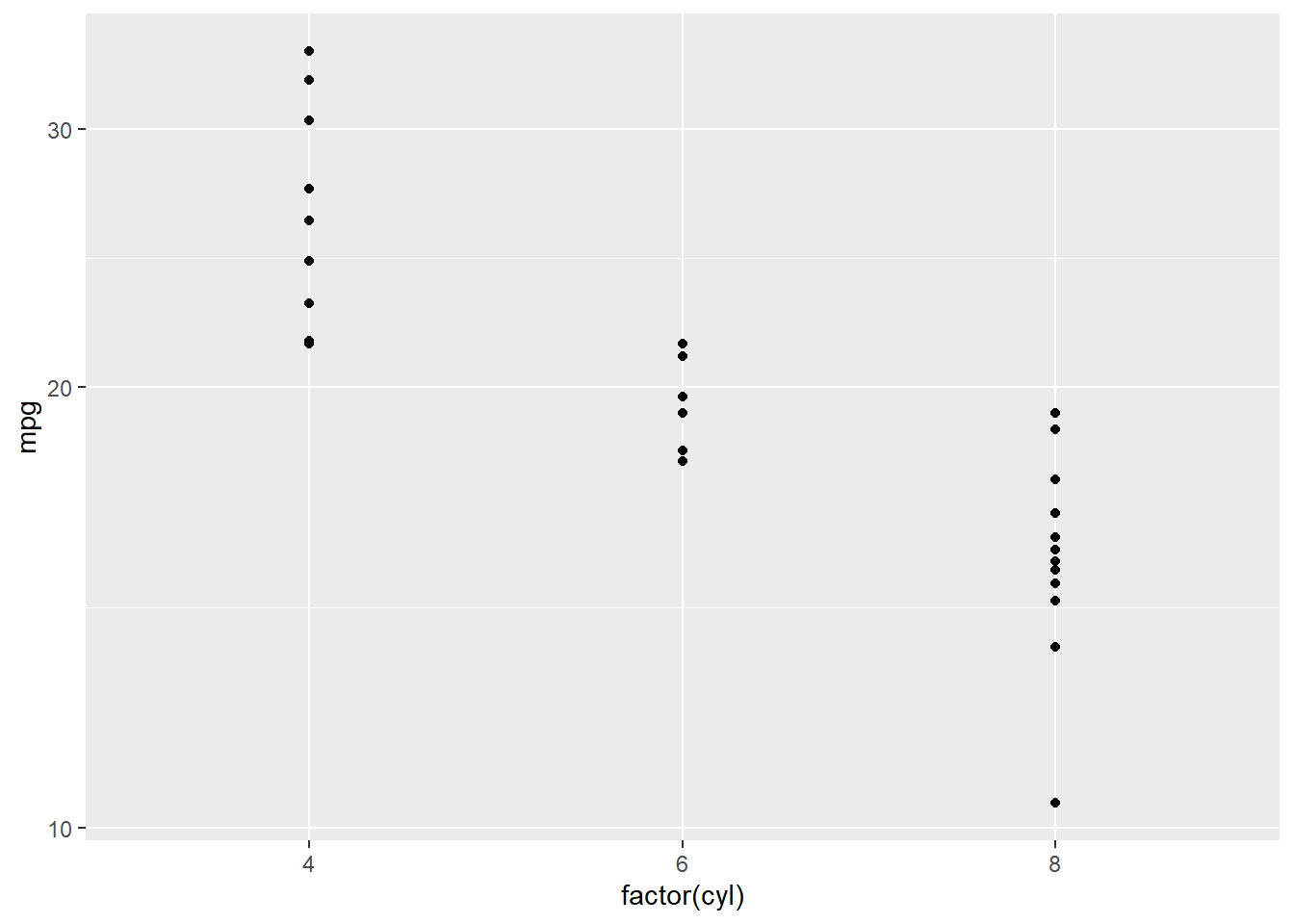
p3 + scale_y_sqrt()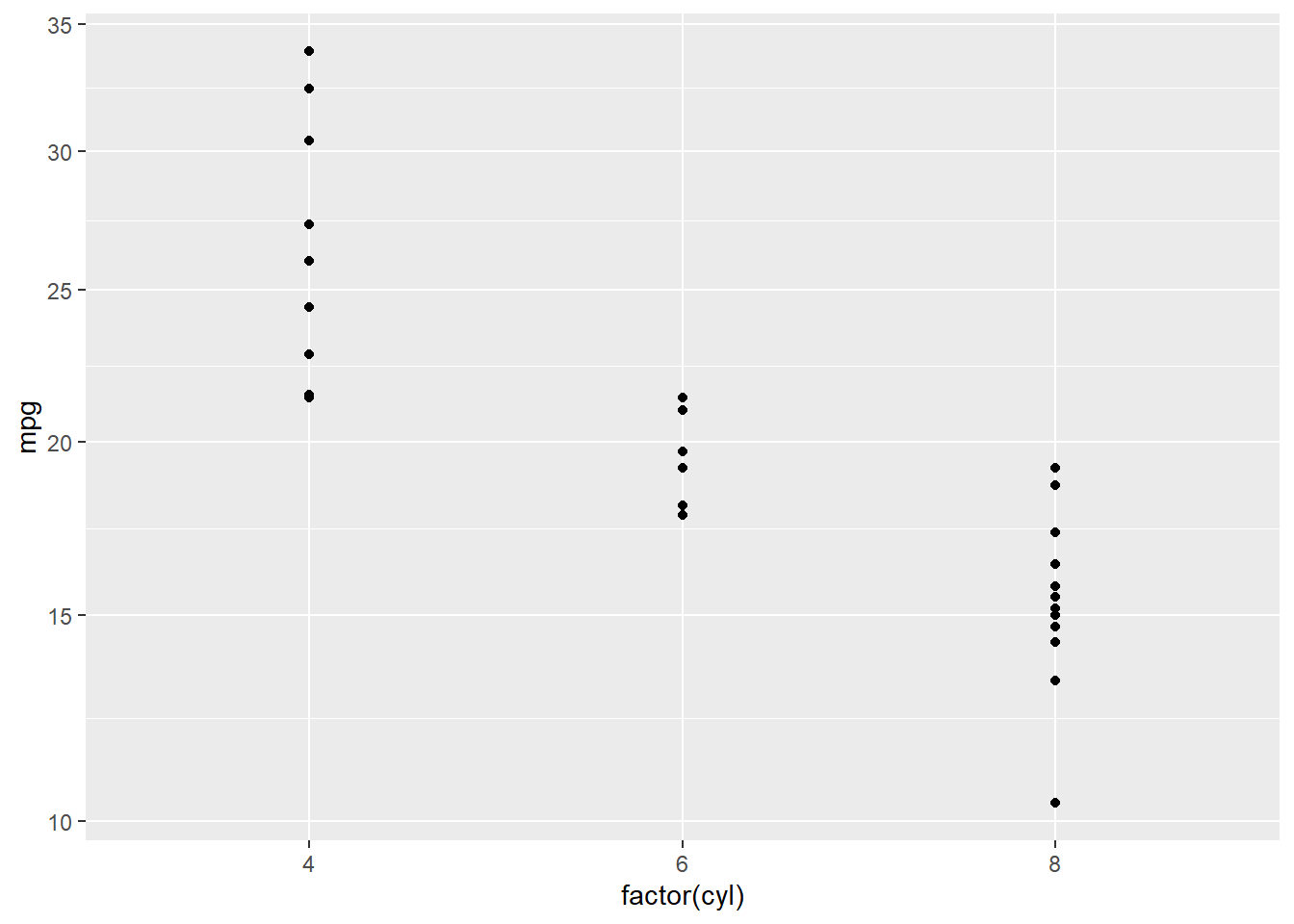
10.2 更改颜色
更改color/fill
10.2.1 离散型 例 1
p0 + scale_fill_manual(values=c("red", "blue", "green")) # 直接指定三个颜色# 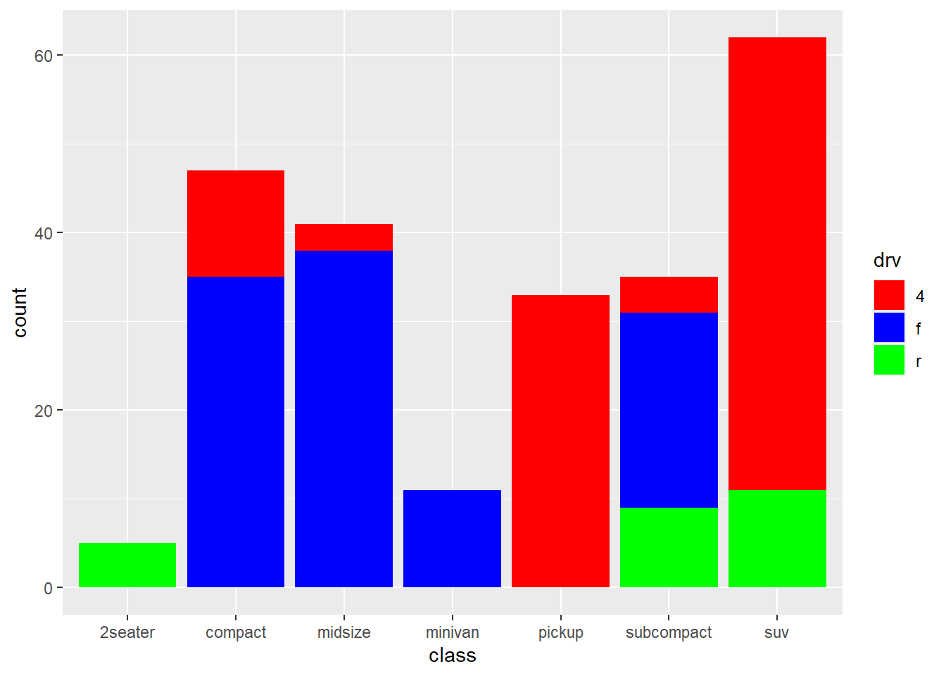
p0 + scale_color_hue(h=c(15,100)) #前面使用fill分组,用color系列无效#
p0 + scale_fill_brewer(palette = "Greens",direction = -1)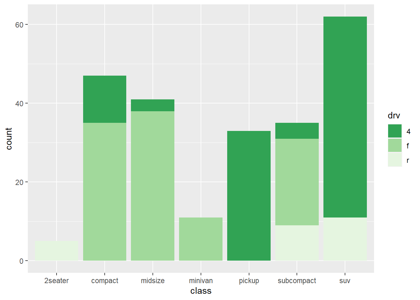
p0 + scale_fill_grey(start=1, end=0.5)#0为黑,1为白#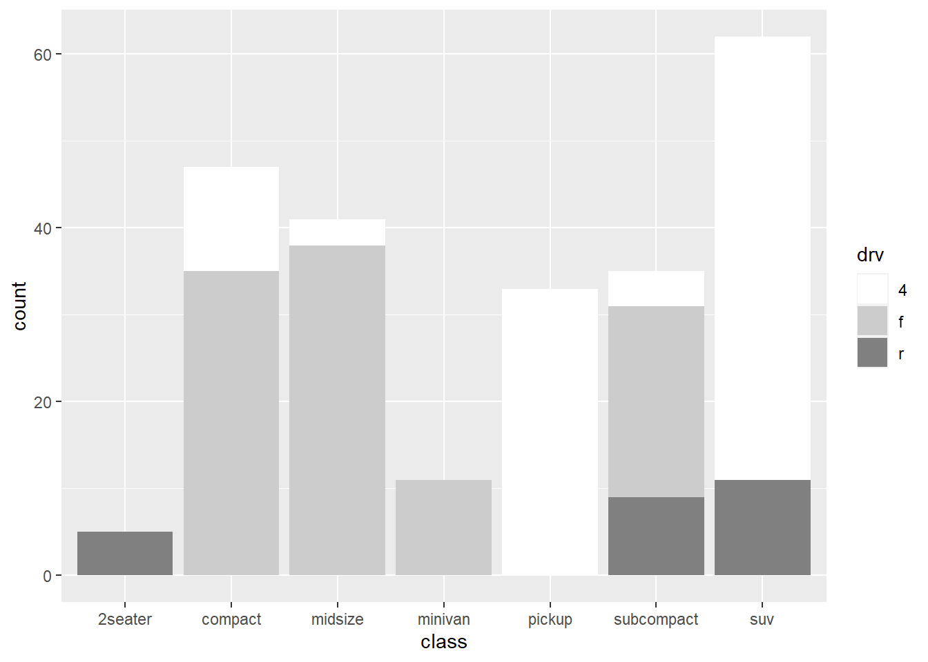
10.2.2 离散型 例 2
x <- sample(LETTERS,13); y <- 1:13
x
[1] "L" "N" "H" "V" "M" "Z" "D" "W" "E" "K" "B" "Q" "G"y [1] 1 2 3 4 5 6 7 8 9 10 11 12 13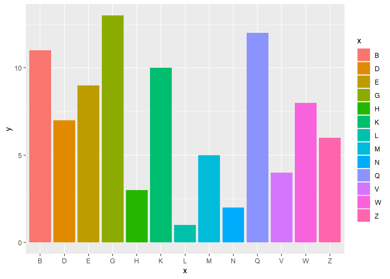
Warning in RColorBrewer::brewer.pal(n, pal): n too large, allowed maximum for palette Blues is 9
Returning the palette you asked for with that many colors
p+scale_fill_brewer(palette="YlOrRd")Warning in RColorBrewer::brewer.pal(n, pal): n too large, allowed maximum for palette YlOrRd is 9
Returning the palette you asked for with that many colors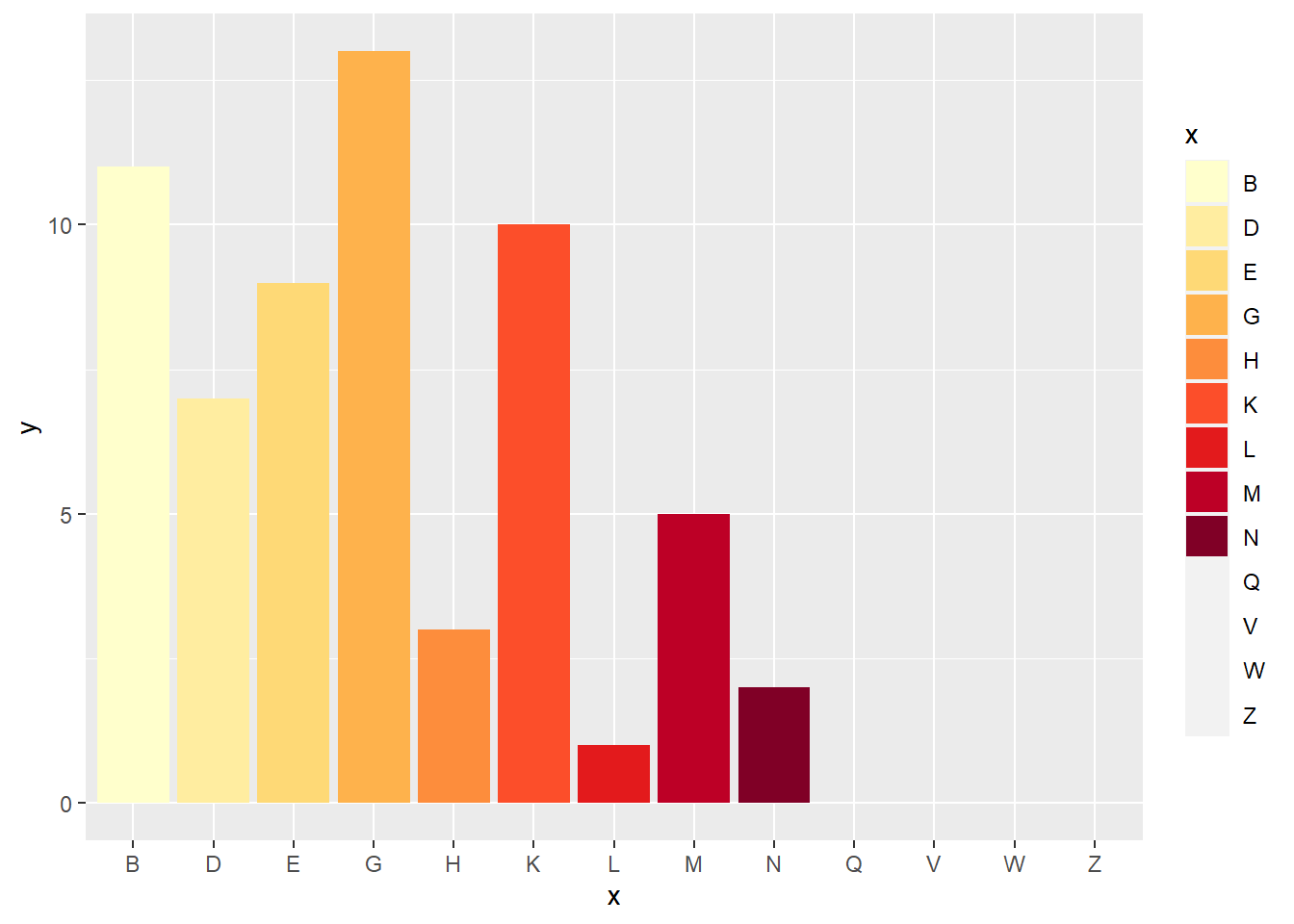
x<-x[1:8];y<-y[1:8]
x
[1] "L" "N" "H" "V" "M" "Z" "D" "W"y[1] 1 2 3 4 5 6 7 8
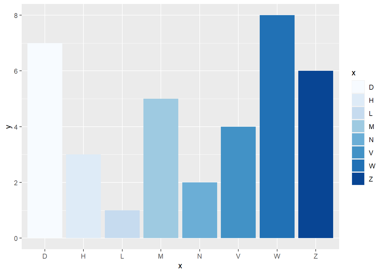
p+scale_fill_brewer(palette="YlOrRd")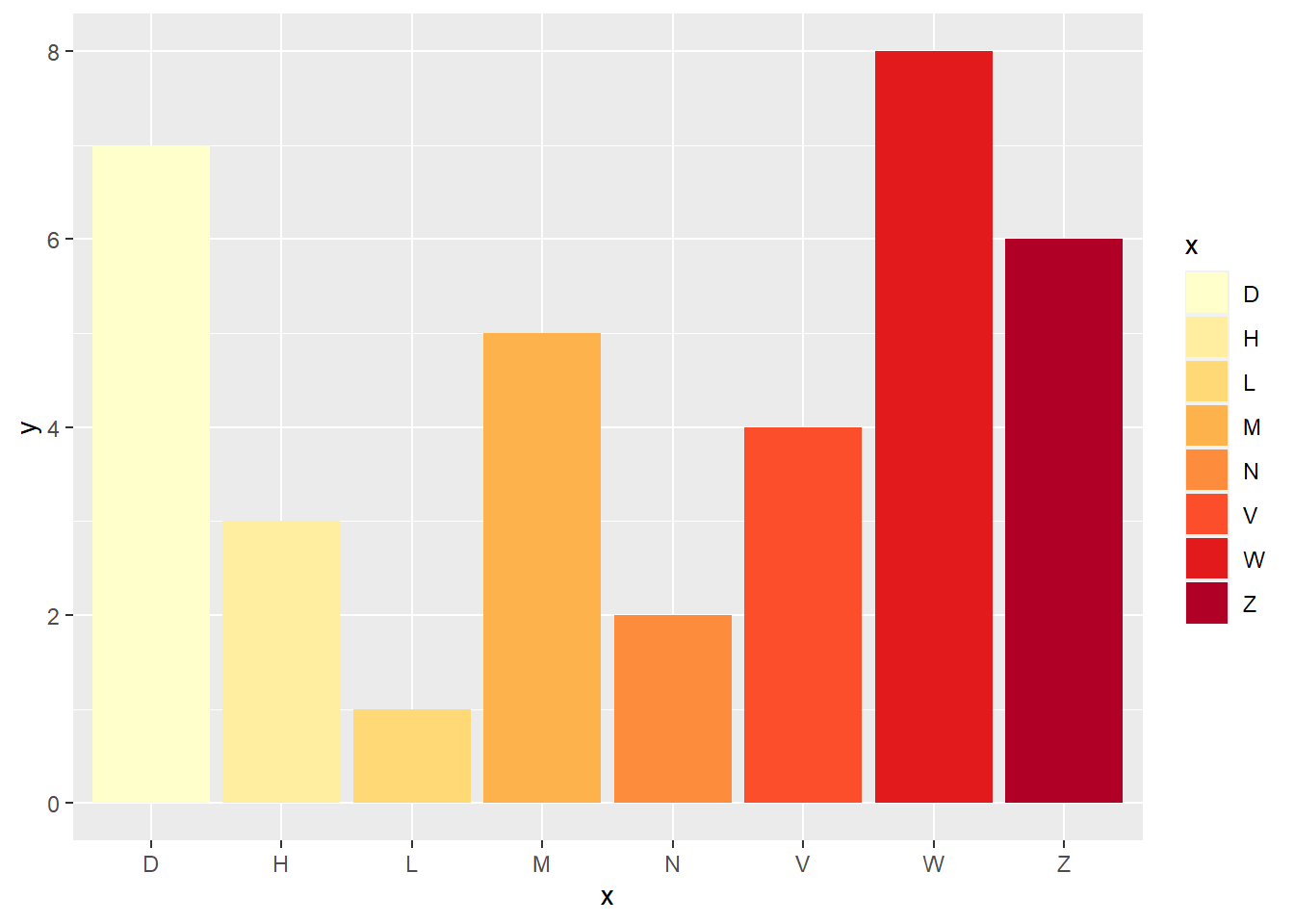
10.2.3 连续型 例 1
p1<-ggplot(mpg,aes(displ, hwy , color = cyl))+geom_point();p1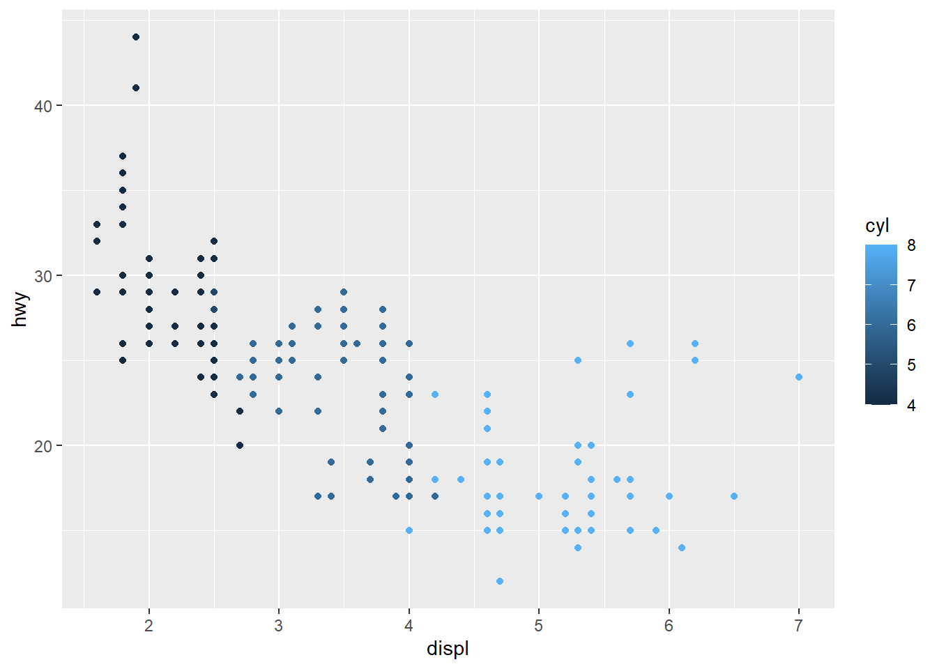
p1 + scale_color_gradient2(low = "white", mid = "red", high = "black") 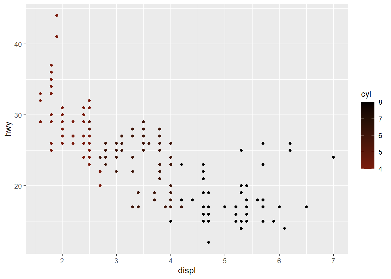
p1 + scale_color_gradientn(colours = terrain.colors(10))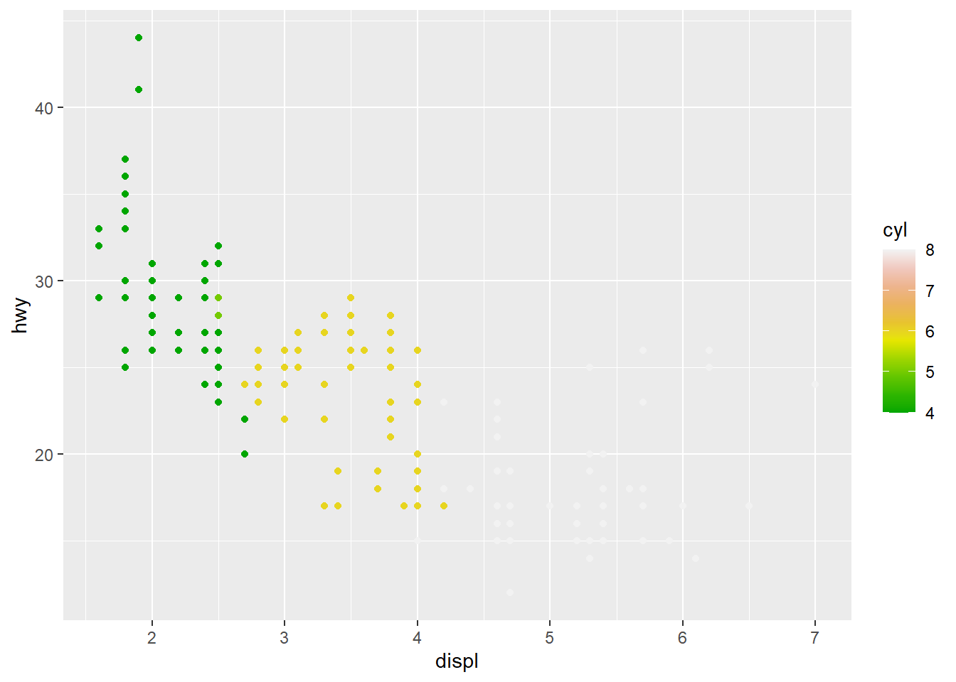
p1 + scale_color_distiller(palette = "Spectral")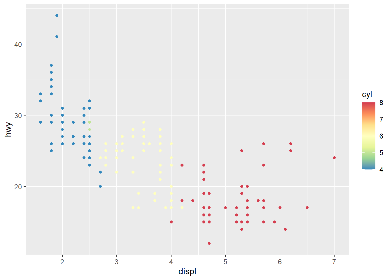
10.2.4 连续型 例 2
p<-ggplot(faithfuld, aes(waiting, eruptions)) + geom_raster(aes(fill = density));p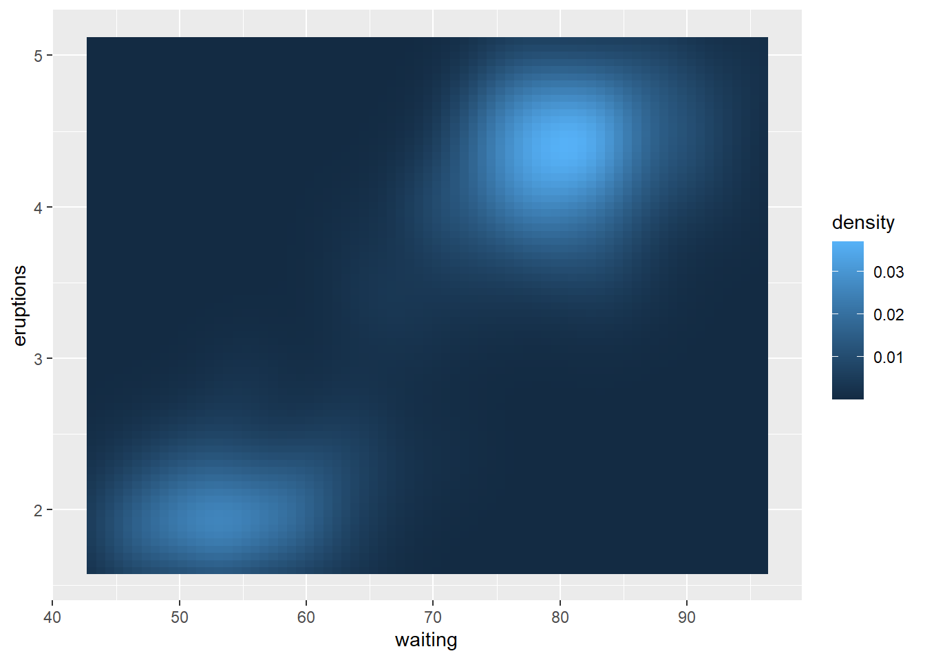
p + scale_fill_gradient(limits=c(0.001,0.004)) 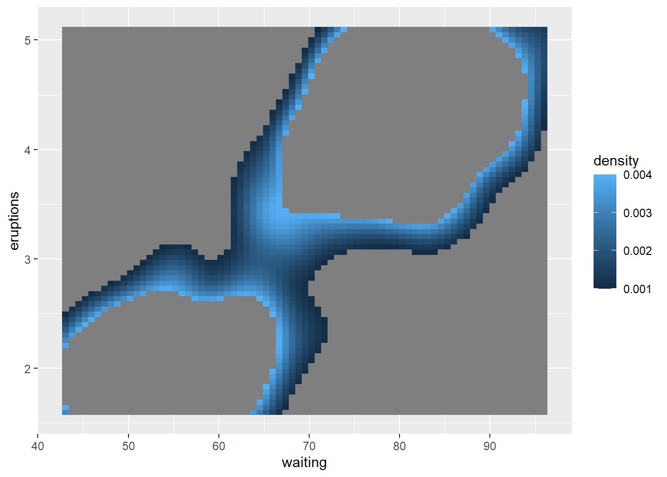
p + scale_fill_gradient(low = 'blue', high = 'red')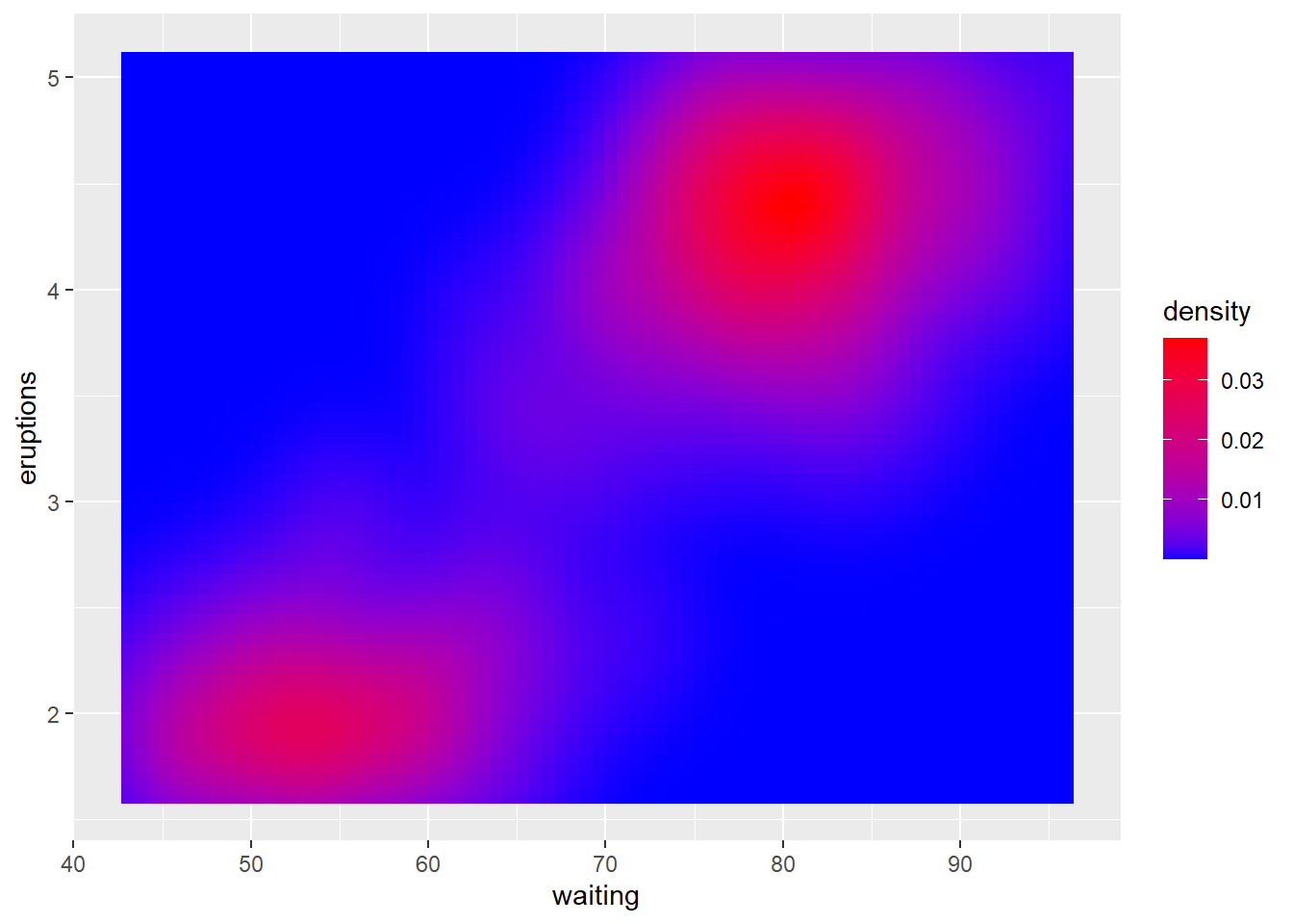
p + scale_fill_gradient2(low = 'blue', high = 'red') 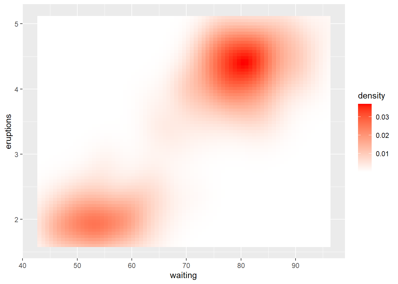
p + scale_fill_gradient2(low = 'blue', high = 'red', midpoint = 0.02)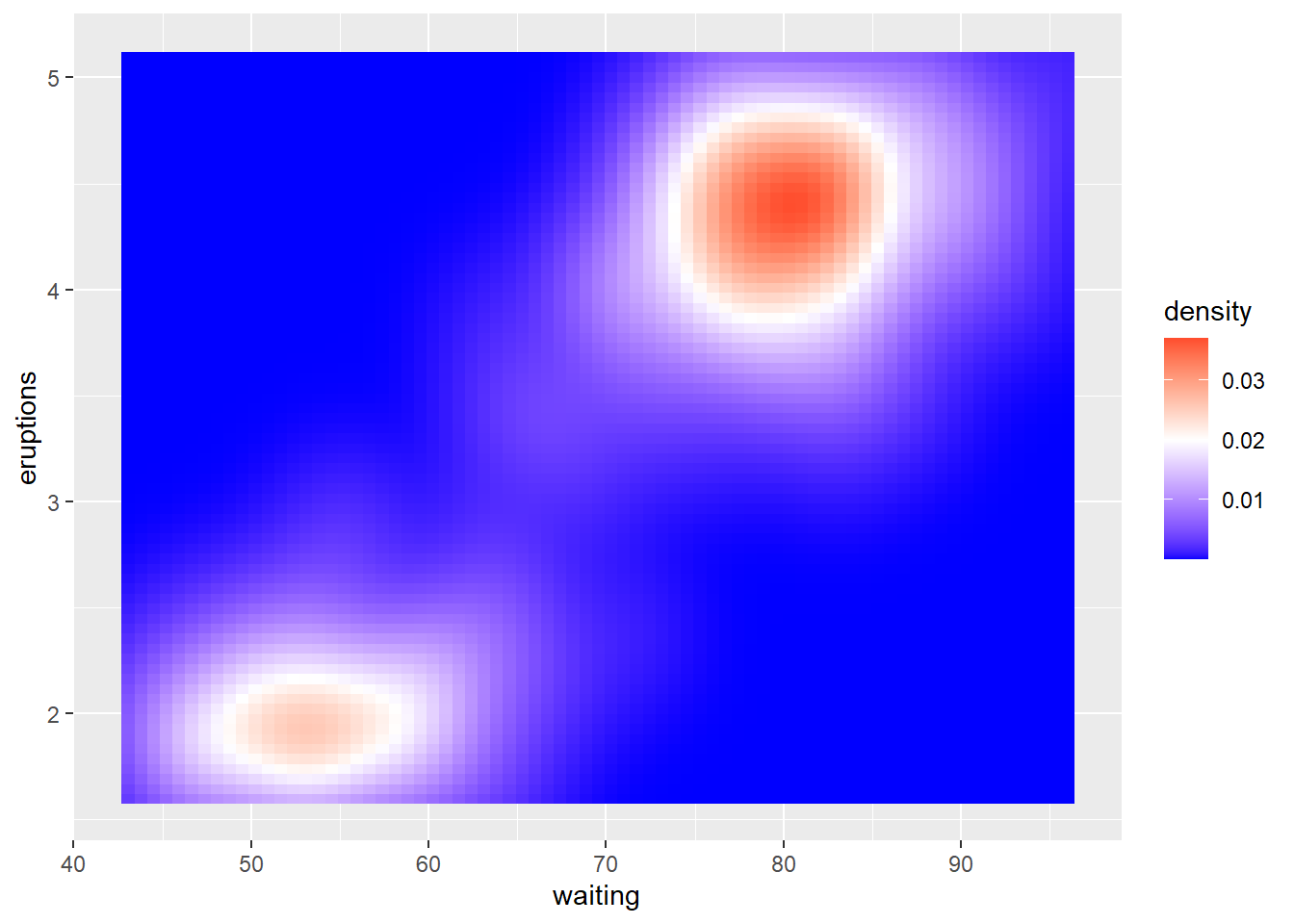
p + scale_fill_gradientn(colours = c('black','blue','red','white')) 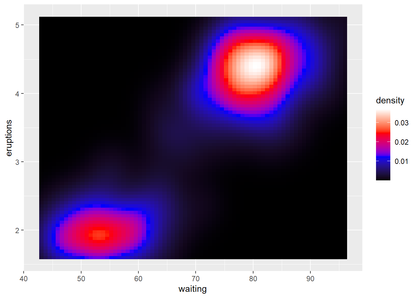
p + scale_fill_gradientn(colours = topo.colors(10)) 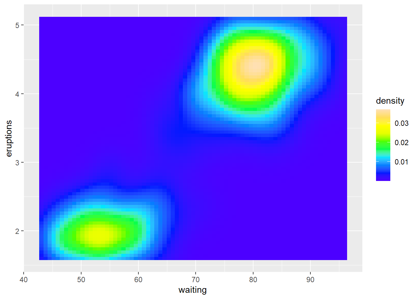
p + scale_fill_gradientn(colours = terrain.colors(10)) 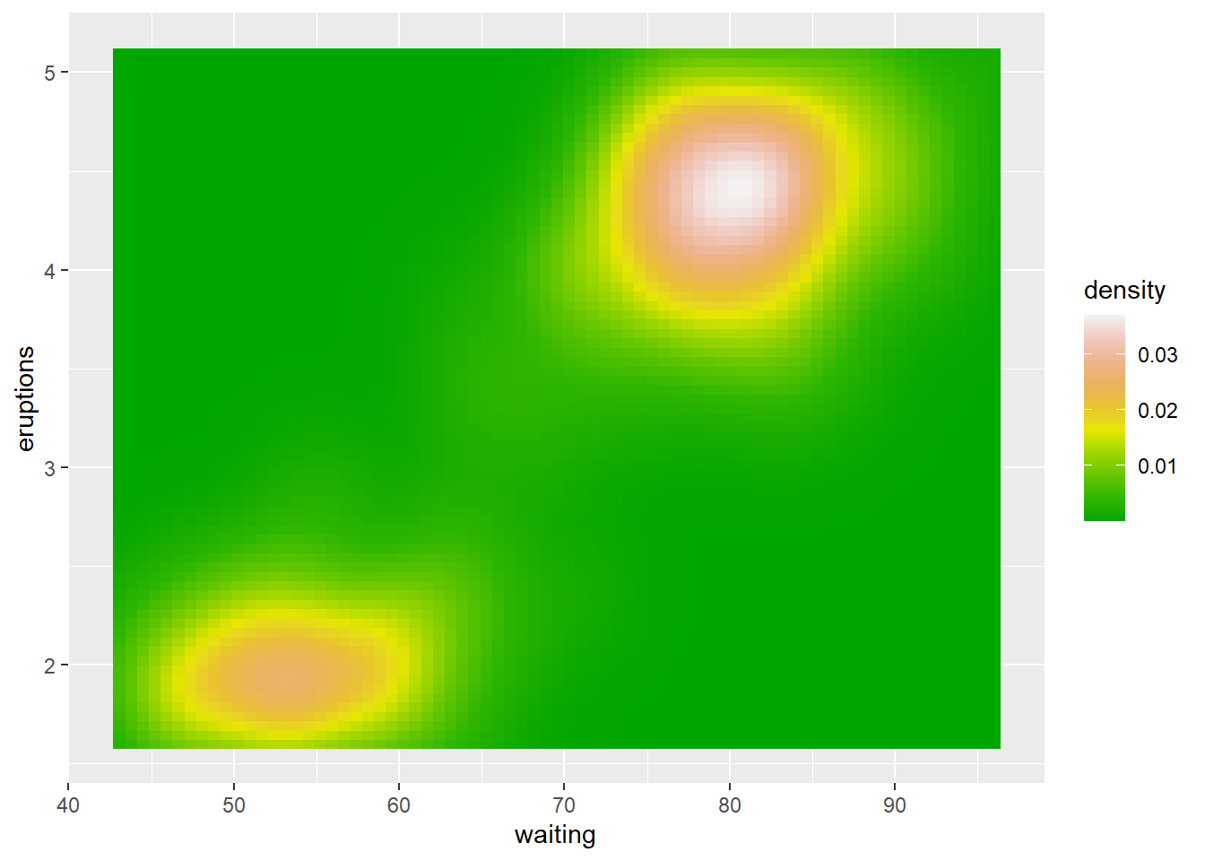
p + scale_fill_gradientn(colours = heat.colors(10))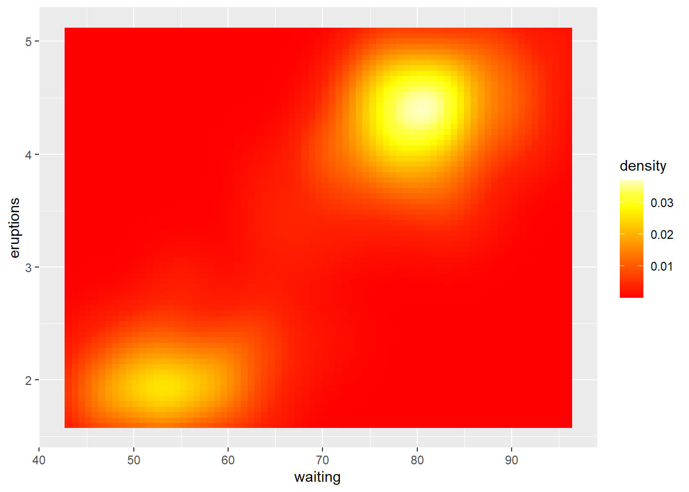
p + scale_fill_gradientn(colours = cm.colors(10))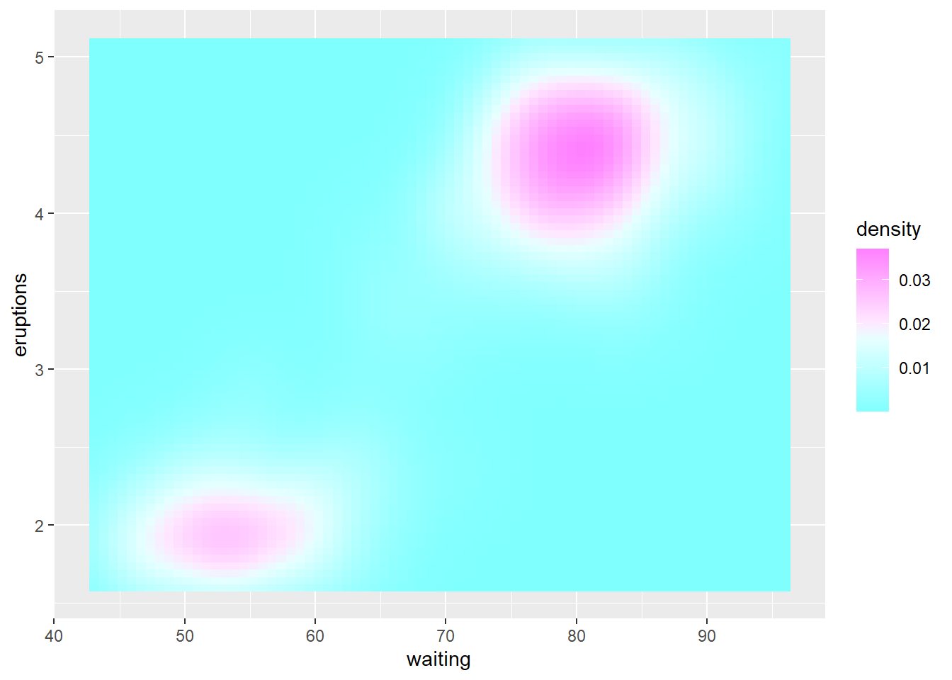
p + scale_fill_distiller(palette = "Spectral")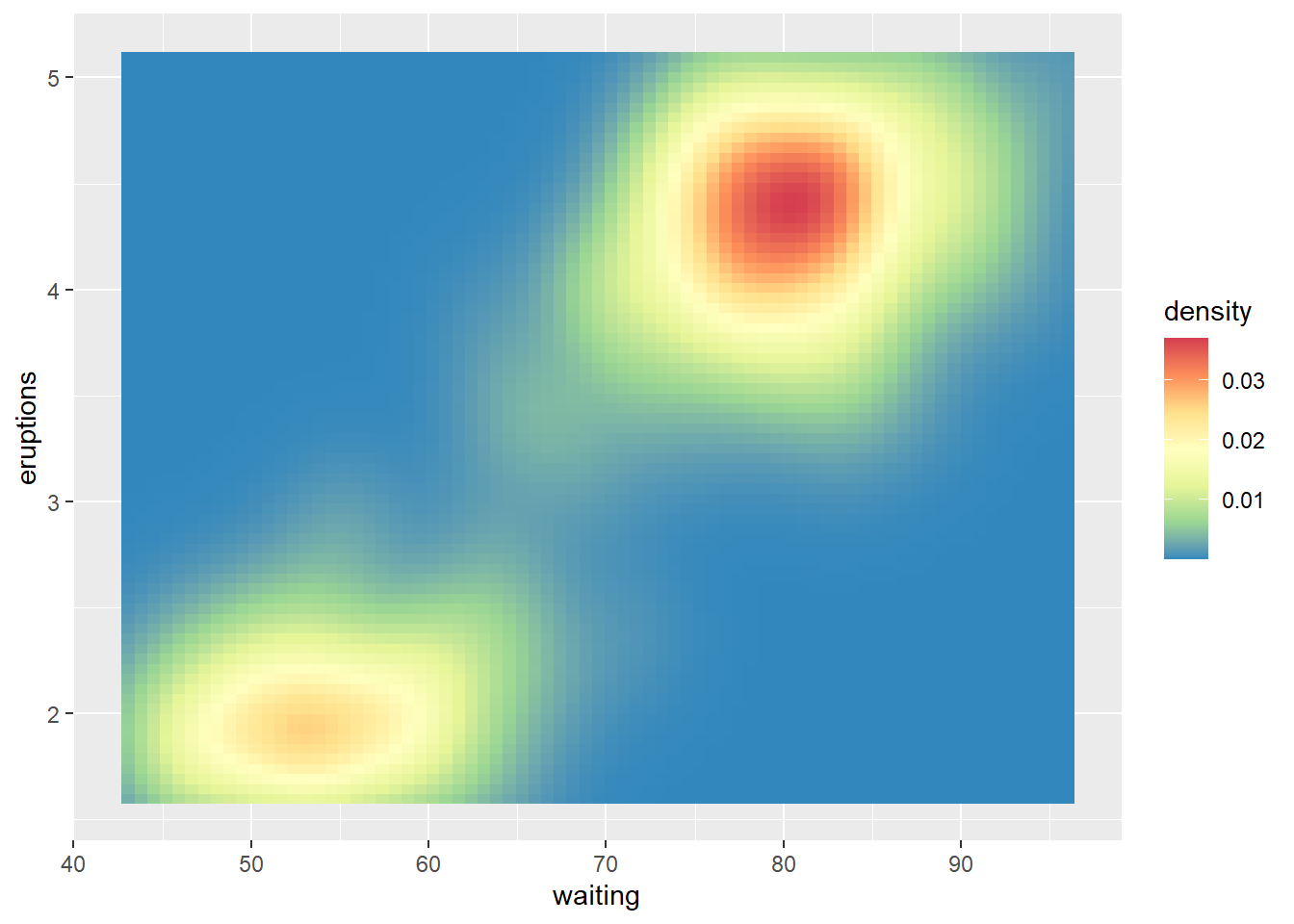
10.3 scale_color_identity()
pp1<-ggplot(mpg,aes(displ, hwy , color = "blue"))+geom_point();pp1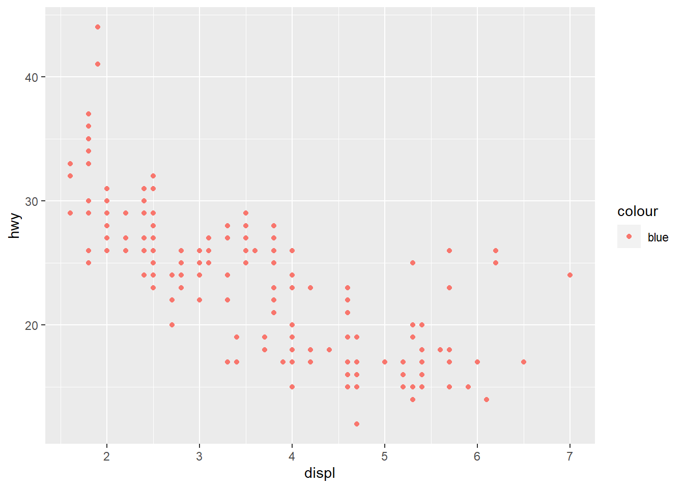
pp1+scale_color_identity( )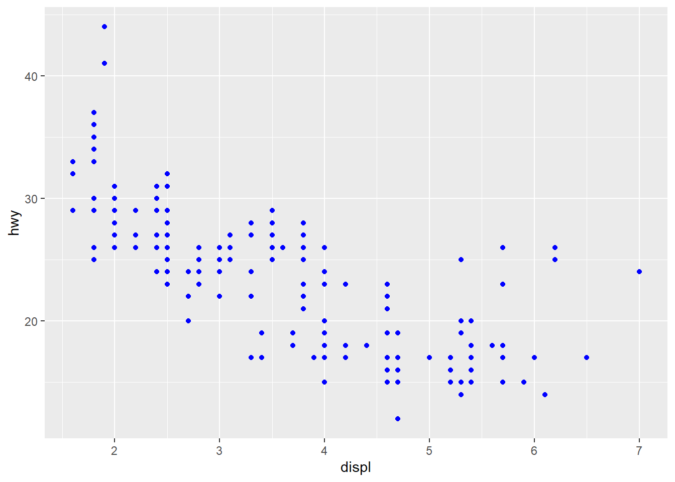
[1] 7.497713 5.036814 14.489637 7.368140data<-data.frame("col"=col,"val"=val)
data col val
1 red 7.497713
2 yellow 5.036814
3 blue 14.489637
4 black 7.368140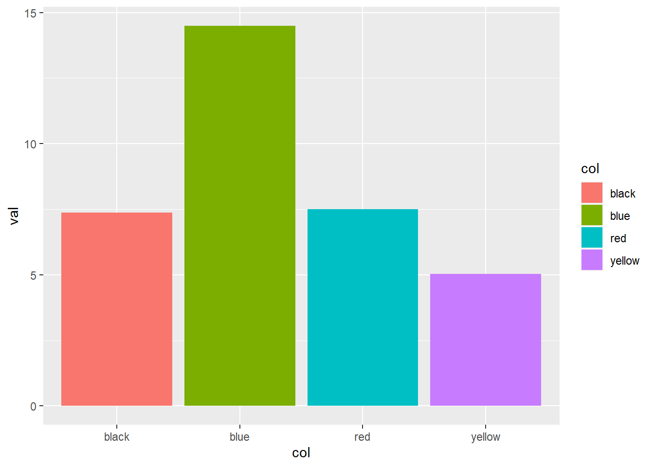
pp2+scale_fill_identity()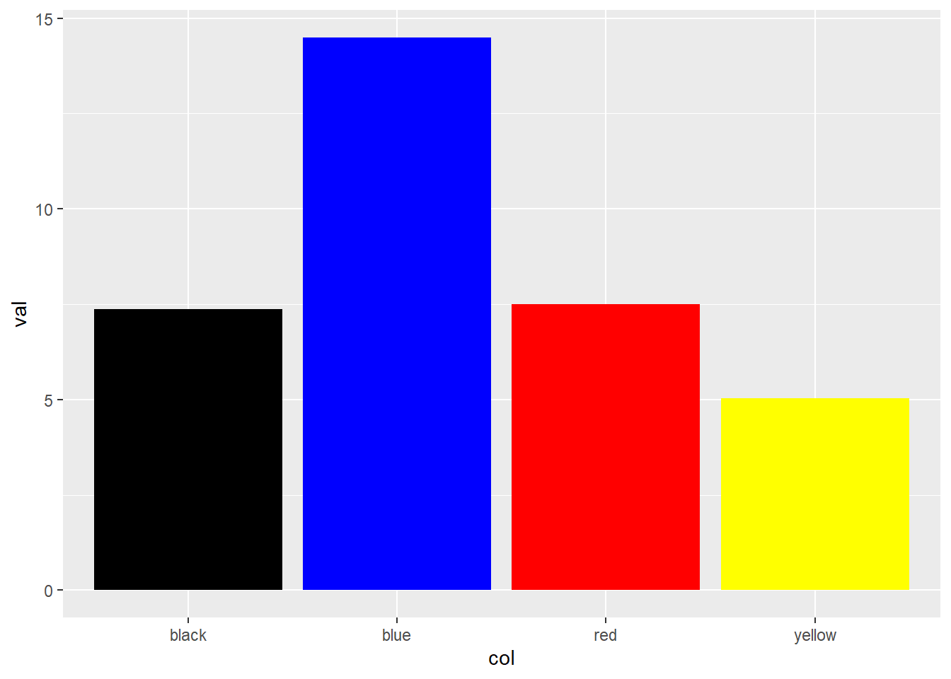
10.4 scale_shape_**()
df_shapes <- data.frame(shape = 0:24)
df_shapes
shape
1 0
2 1
3 2
4 3
5 4
6 5
7 6
8 7
9 8
10 9
11 10
12 11
13 12
14 13
15 14
16 15
17 16
18 17
19 18
20 19
21 20
22 21
23 22
24 23
25 24ggplot(df_shapes, aes(0, 0, shape = shape)) +
geom_point(aes(shape = shape), size = 5, fill = 'red') +
scale_shape_identity() +
facet_wrap(~shape)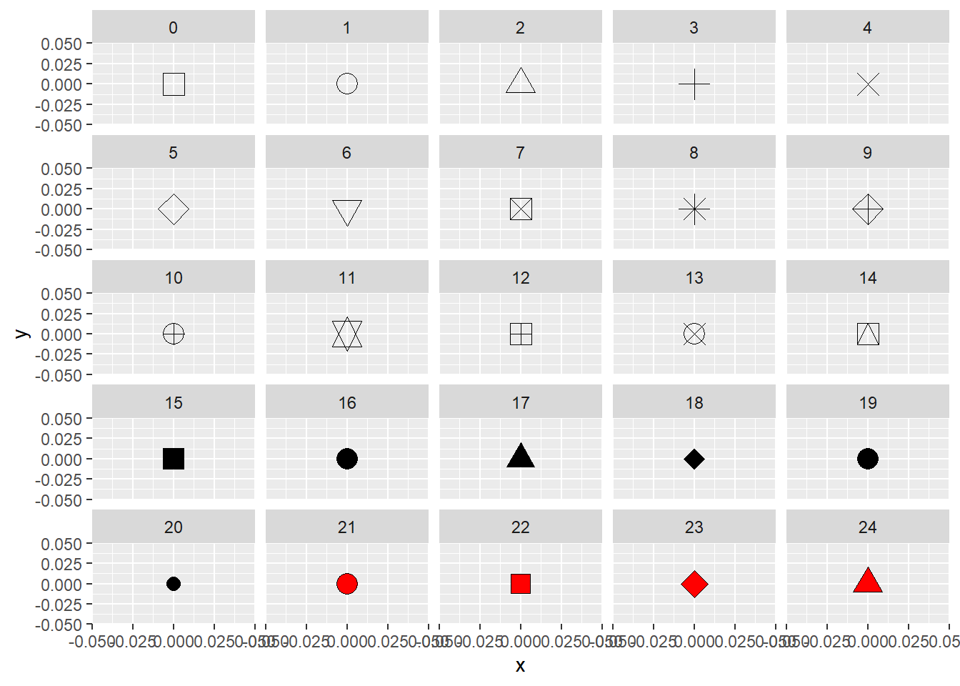
p<-ggplot(mpg)+
   geom_point(aes(cty, hwy, shape = manufacturer));p
Warning: The shape palette can deal with a maximum of 6 discrete values because
more than 6 becomes difficult to discriminate; you have 15. Consider
specifying shapes manually if you must have them.Warning: Removed 112 rows containing missing values (geom_point).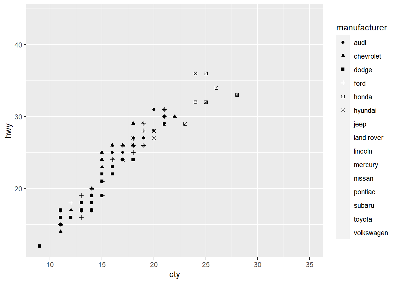
p+ scale_shape_manual(values=seq(1,15,1))
10.5 scale_linetype_**()
df_lines <- data.frame(
    linetype = factor(
        1:4,
        labels = c("solid", "longdash", "dashed", "dotted")
    )
)
df_lines
linetype
1 solid
2 longdash
3 dashed
4 dottedggplot(df_lines) +
geom_hline(aes(linetype = linetype, yintercept = 0), size = 2) +
scale_linetype_identity() +
facet_grid(linetype ~ .) 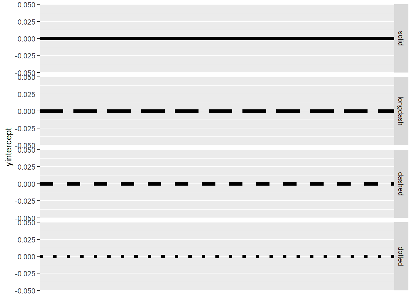
df_lines <- data.frame(
    linetype = factor(
        1:13,
        labels = as.character(seq(0,12,1))
    )
)
ggplot(df_lines) +
    geom_hline(aes(linetype = linetype, yintercept = 0), size = 2) +
facet_grid(linetype ~ .) 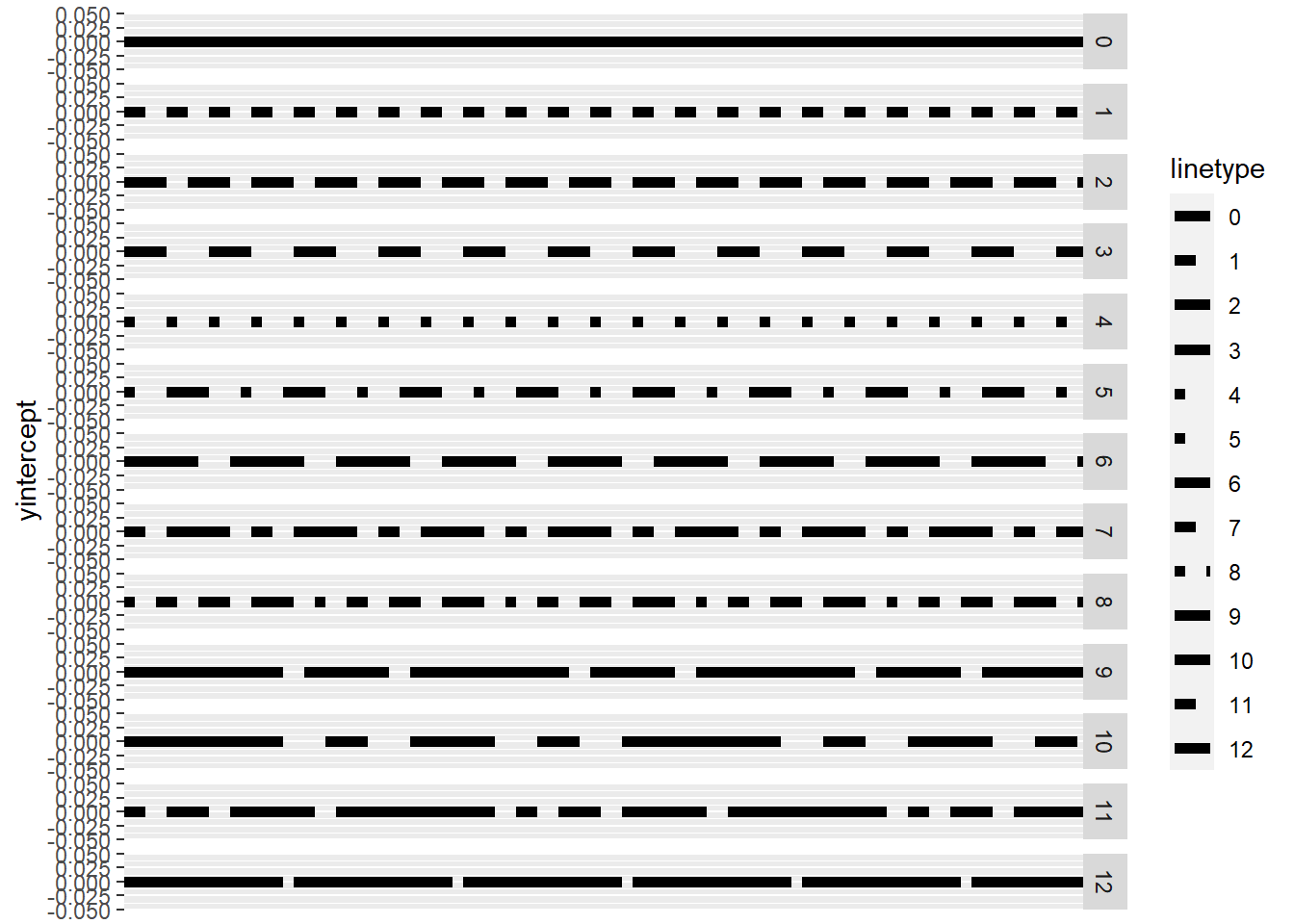
10.6 scale_size_**()
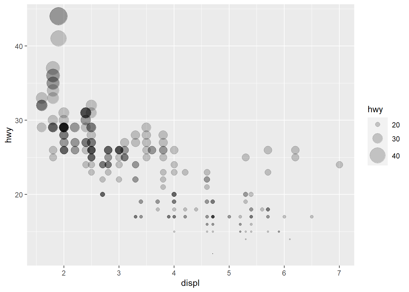
p<-ggplot(mpg)+
   geom_point(aes(displ, hwy, size = hwy),alpha=0.2);p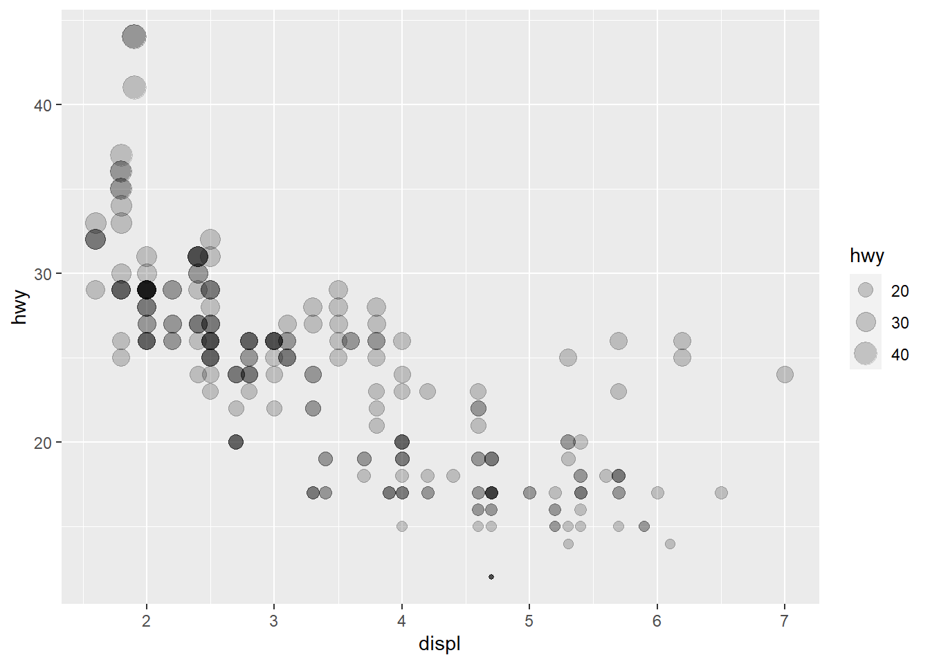
p+ scale_size()
p+scale_size(range=c(0,10))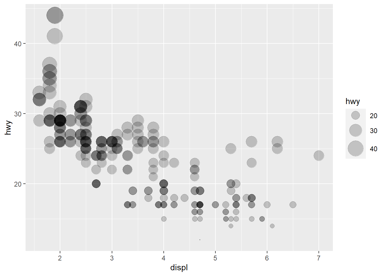
p+scale_size_area(max_size=10)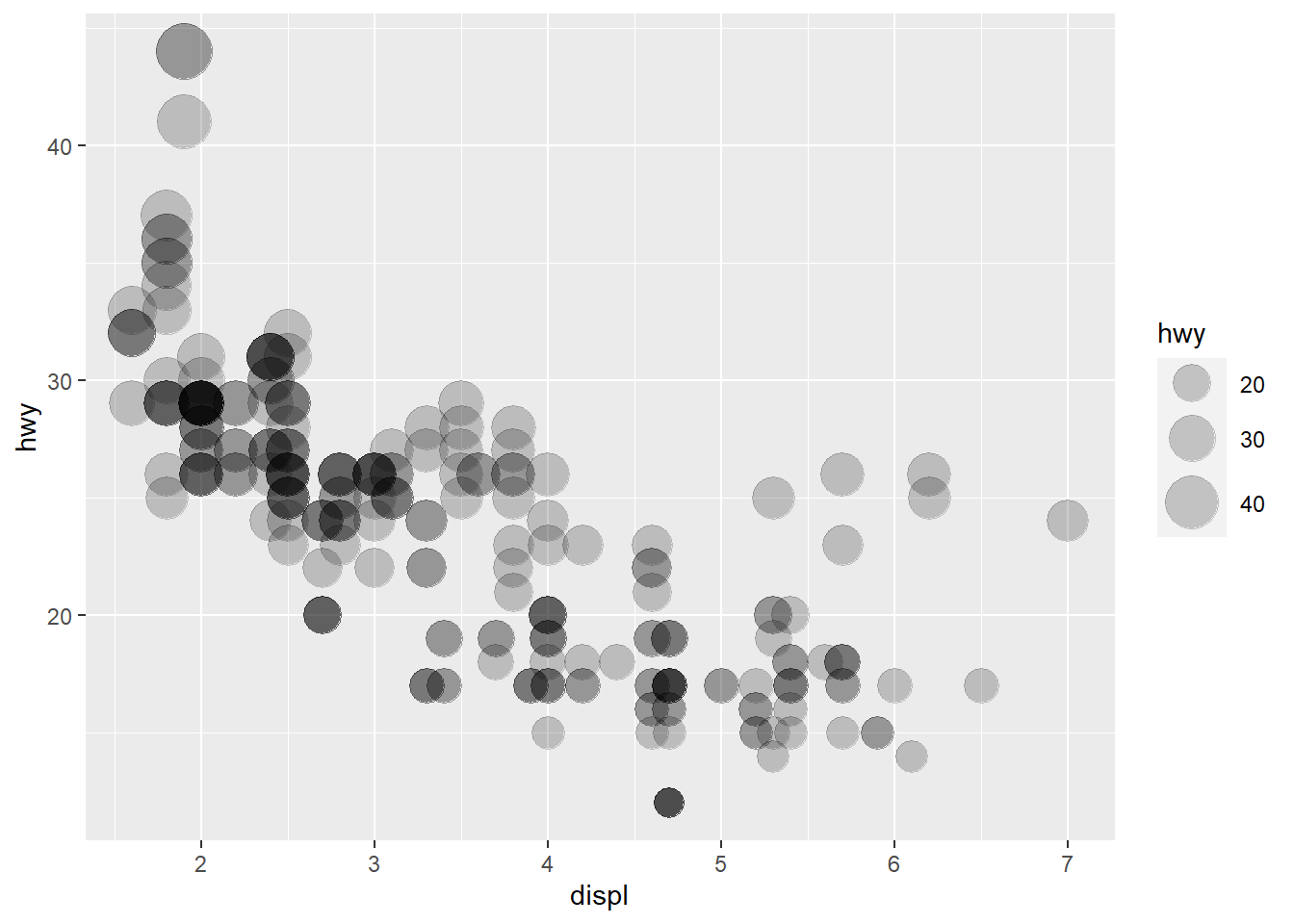
p+scale_radius(range=c(0,10))