15 multiplot

library(easyGgplot2)
library(gridExtra)
library(grid)
library(tidyverse)

15.1 easyGgplot2

remotes::install_github(“kassambara/easyGgplot2”)

df <- ToothGrowth # 自定义框图与中心点图
as_tibble(df)

# A tibble: 60 × 3
     len supp   dose
   <dbl> <fct> <dbl>
 1   4.2 VC      0.5
 2  11.5 VC      0.5
 3   7.3 VC      0.5
 4   5.8 VC      0.5
 5   6.4 VC      0.5
 6  10   VC      0.5
 7  11.2 VC      0.5
 8  11.2 VC      0.5
 9   5.2 VC      0.5
10   7   VC      0.5
# … with 50 more rows

Code

plot1<-ggplot2.boxplot(data=df, xName='dose',yName='len', 
                       groupName='dose', addDot=TRUE, 
                       dotSize=1, showLegend=FALSE) # 带中心点图的自定义点图 
plot2<-ggplot2.dotplot(data=df, xName='dose',yName='len', 
                       groupName='dose',showLegend=FALSE) # 带有中心点图的自定义带状图 
plot3<-ggplot2.stripchart(data=df, xName='dose',yName='len', 
                          groupName='dose', showLegend=FALSE) # Notched box plot 
plot4<-ggplot2.boxplot(data=df, xName='dose',yName='len', 
                       notch=TRUE) #在同一页上的多个图表 
ggplot2.multiplot(plot1,plot2,plot3,plot4, cols=2)

15.2 gridExtra

df <- ToothGrowth # 自定义框图与中心点图
as_tibble(df)

# A tibble: 60 × 3
     len supp   dose
   <dbl> <fct> <dbl>
 1   4.2 VC      0.5
 2  11.5 VC      0.5
 3   7.3 VC      0.5
 4   5.8 VC      0.5
 5   6.4 VC      0.5
 6  10   VC      0.5
 7  11.2 VC      0.5
 8  11.2 VC      0.5
 9   5.2 VC      0.5
10   7   VC      0.5
# … with 50 more rows

Code

plot1<-ggplot2.boxplot(data=df, xName='dose',yName='len', 
                       groupName='dose', addDot=TRUE, dotSize=1, 
                       showLegend=FALSE) # 带中心点图的自定义点图 
plot2<-ggplot2.dotplot(data=df, xName='dose',yName='len', 
                       groupName='dose',
                       showLegend=FALSE) # 带有中心点图的自定义带状图 
plot3<-ggplot2.stripchart(data=df, xName='dose',yName='len', 
                          groupName='dose', 
                          showLegend=FALSE) # Notched box plot 
plot4<-ggplot2.boxplot(data=df, xName='dose',yName='len', 
                       notch=TRUE) #在同一页上的多个图表
grid.arrange(plot1,plot2,plot3,plot4, ncol=2)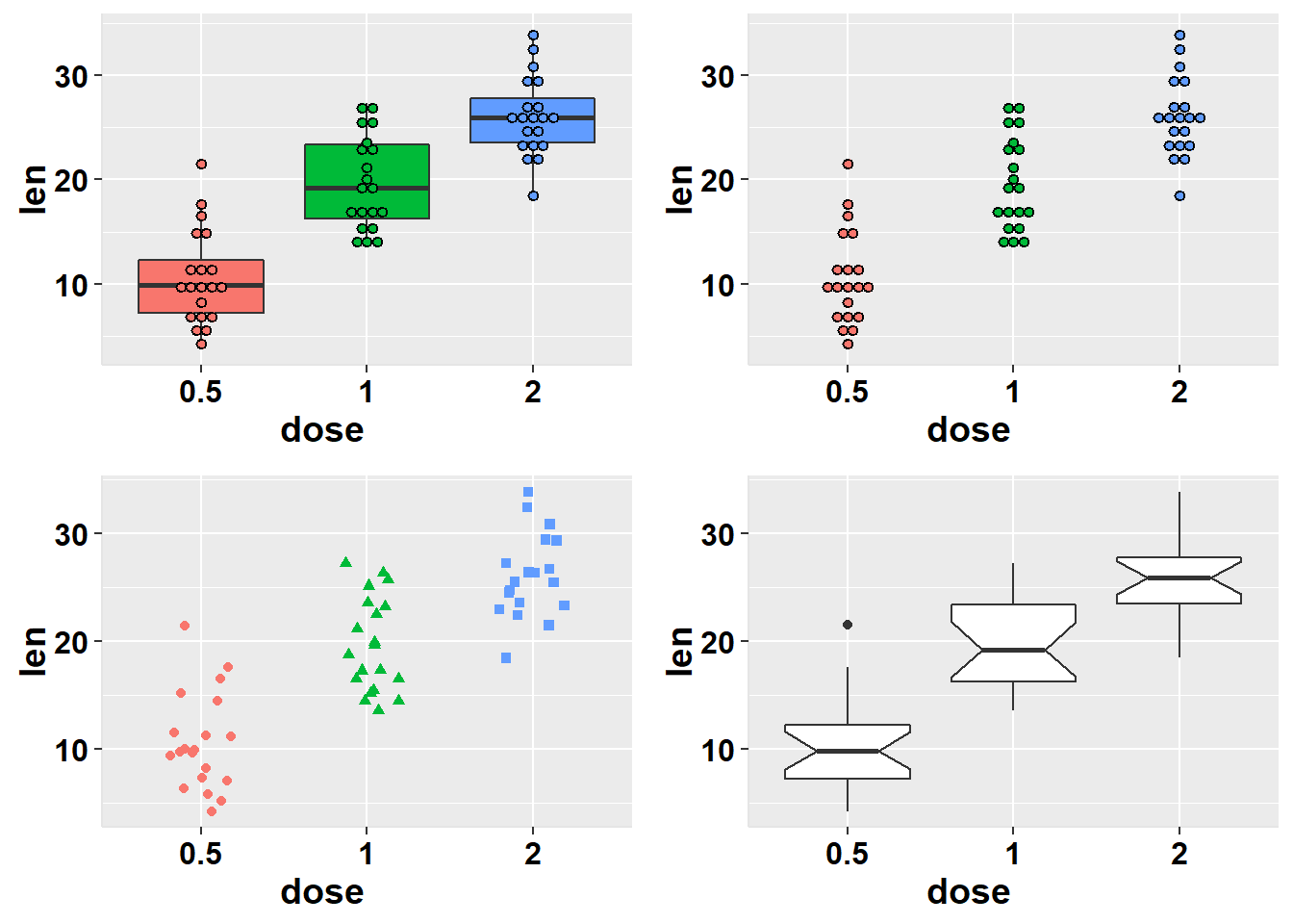

15.3 grid

Code

#####先将图画好，并且赋值变量，储存#####
a <- ggplot(mtcars, aes(mpg, wt, colour = factor(cyl))) + geom_point()
b <- ggplot(diamonds, aes(carat, depth, colour = color)) + geom_point()
c <- ggplot(diamonds, aes(carat, depth, colour = color)) + geom_point() + 
  facet_grid(.~color,scale = "free") 

########新建画图页面###########
grid.newpage()  ##新建页面
pushViewport(viewport(layout = grid.layout(2,2))) ####将页面分成2*2矩阵
vplayout <- function(x,y){
  viewport(layout.pos.row = x, layout.pos.col = y)
}
print(c, vp = vplayout(1,1:2))   ###将（1,1)和(1,2)的位置画图c
print(b, vp = vplayout(2,1))   ###将(2,1)的位置画图b
print(a, vp = vplayout(2,2))  ###将（2,2)的位置画图a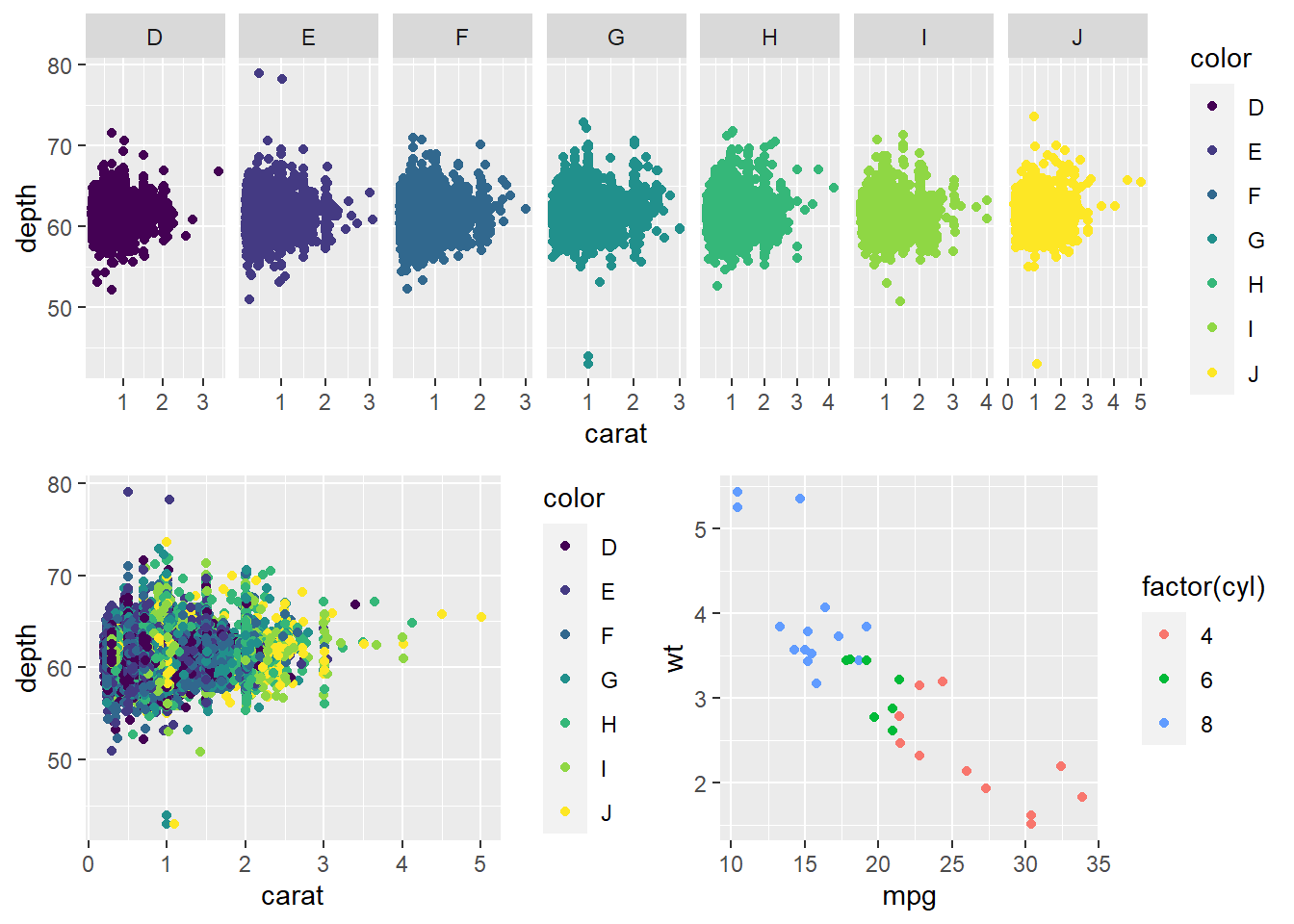

Code

#dev.off() ##画下一幅图，记得关闭窗口

15.3.1 子母图viewplot

Code

library(grid)
a <- ggplot(diamonds, aes(carat, depth, colour = color)) + geom_point()
b <- ggplot(mtcars, aes(mpg, wt, colour = factor(cyl))) + geom_point()
subvp <- viewport(x = 0.8, y = 0.8, width = 0.4, height = 0.4)
a
print(b,vp=subvp)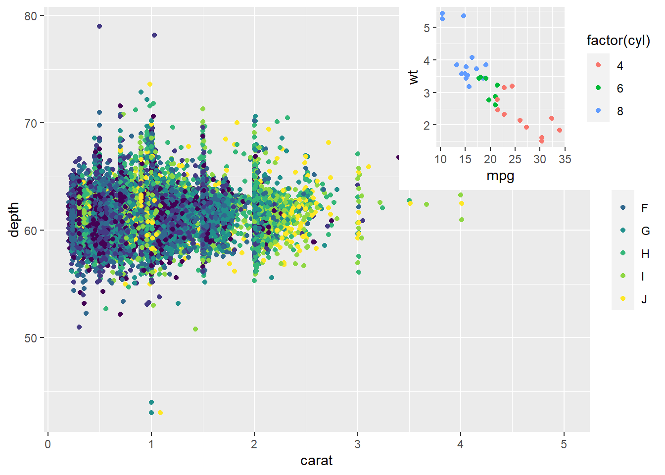

Code

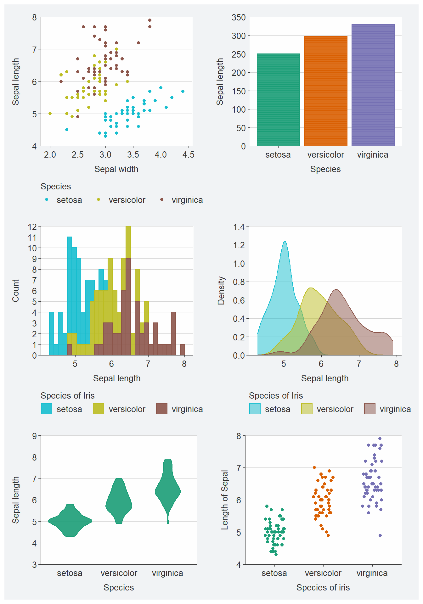
#dev.off()

15.4 patchwork

library(ggblanket)
library(ggplot2) 
library(patchwork) # 拼图
library(pals) # 颜色

Code

p1 <- gg_point(data = iris, 
               x = Sepal.Width, 
               y = Sepal.Length, 
               col = Species)
 
p2 <- gg_bar(data = iris, 
             x = Species, 
             y = Sepal.Length, 
             col = Species, 
             stat = "identity", 
             pal = brewer.dark2(3))
 
p3 <- gg_histogram(data = iris, 
                   x = Sepal.Length, 
                   col = Species, 
                   col_title = "Species of Iris", 
                   y_breaks = scales::breaks_width(1))
 
p4 <- gg_density(data = iris, 
                 x = Sepal.Length, 
                 col = Species, 
                 col_title = "Species of Iris")
 
p5 <- gg_violin(iris, 
                x = Species, 
                y = Sepal.Length, 
                y_include = c(3, 9), # y轴范围
                pal = brewer.dark2(3)) 
 
p6 <- gg_jitter(iris, 
                x = Species, 
                y = Sepal.Length, 
                col = Species, 
                y_title = "Length of Sepal", 
                x_title = "Species of iris", 
                position = position_jitter(width = 0.2, height = 0, seed = 123), 
                pal = brewer.dark2(3))

(p1+p2)/(p3+p4)/(p5+p6)# 拼图

`stat_bin()` using `bins = 30`. Pick better value with `binwidth`.