16  Example

16.1 画房子

16.1.1 方法 1

Code
library(tidyverse)
ggplot()+
  scale_x_continuous(name=NULL,breaks=NULL,label=NULL,limits=c(0,1000))+
  scale_y_continuous(name=NULL,breaks=NULL,label=NULL,limits=c(0,1000))+
  theme(panel.background = element_rect(fill="white"))+
  coord_fixed()+
  geom_polygon(aes(x=c(200,700,700,200),y=c(50,50,600,600)),fill="brown",color="white")+
  geom_polygon(aes(x=c(50,450,850),y=c(600,830,600)),color="black",fill="black")+
  geom_polygon(aes(c(300,450,450,300),c(50,50,350,350)),fill="orange",color="white")+
  geom_polygon(aes(c(375,380,380,375),c(50,50,350,350)),fill="grey",color="white")+
  geom_polygon(aes(c(355,400,400,355),c(200,200,204,204)),fill="black")+
  geom_point(aes(x=c(391,365),y=c(196,196)),shape=1,size=2)+
  geom_polygon(aes(x=c(500,650,650,500),y=c(400,400,550,550)),fill="white",color="white")+
  geom_point(aes(x=575,y=475),shape=1,size=rel(18),color="red")+
  geom_polygon(aes(x=c(575,576,576,575),y=c(400,400,550,550)),color="black")+
  geom_polygon(aes(x=c(500,650,650,500),y=c(475,475,476,476)),color="black")+
  geom_polygon(aes(x=c(620,670,670,620),y=c(620,620,800,800)),fill="black",color="black")+
  geom_polygon(aes(x=40*sin(seq(-10,10,0.01))+700,y=18*cos(seq(-10,10,0.01))+850),fill="grey",color="black")+
  geom_polygon(aes(x=30*sin(seq(-10,10,0.01))+800,y=14*cos(seq(-10,10,0.01))+900),fill="grey",color="black")

library(readxl)
data <- read_excel("data/data.xlsx",1)
data
# A tibble: 38 × 7
      ID label type      x     y fill   color
   <dbl> <chr> <chr> <dbl> <dbl> <chr>  <chr>
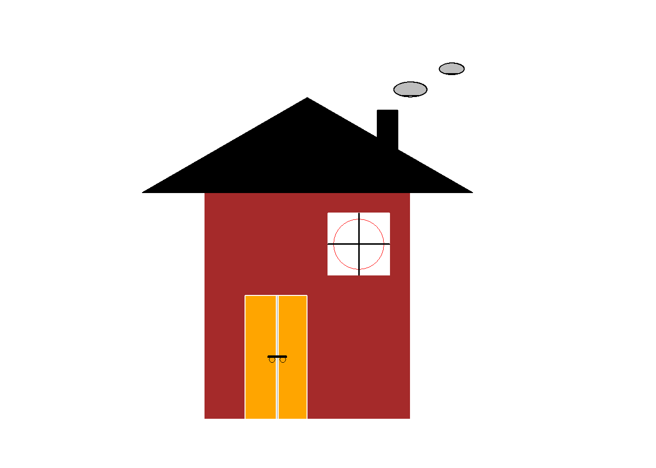
 1     1 墙    qiang   200    50 brown  white
 2     1 墙    qiang   700    50 brown  white
 3     1 墙    qiang   700   600 brown  white
 4     1 墙    qiang   200   600 brown  white
 5     2 房顶  ding     50   600 black  black
 6     2 房顶  ding    450   830 black  black
 7     2 房顶  ding    850   600 black  black
 8     3 门    men     300    50 orange white
 9     3 门    men     450    50 orange white
10     3 门    men     450   350 orange white
# … with 28 more rows

16.1.2 方法 2

Code
library(tidyverse)
ggplot(data=NULL,aes(x,y,fill=fill,color=color))+
  scale_x_continuous(name=NULL,breaks=NULL,label=NULL,limits=c(0,1000))+
  scale_y_continuous(name=NULL,breaks=NULL,label=NULL,limits=c(0,1000))+
  scale_fill_identity()+
  scale_color_identity()+
  theme(panel.background = element_rect(fill="white"))+
  coord_fixed()+
  geom_polygon(data=data[which(data$type=="qiang"),])+   #墙
  geom_polygon(data=data[which(data$type=="ding"),])+    #房顶
  geom_polygon(data=data[which(data$type=="men"),])+     #门
  geom_polygon(data=data[which(data$type=="menfeng"),])+ #门缝
  geom_polygon(data=data[which(data$type=="menshuan"),])+#门栓
  geom_point(data=data[which(data$type=="menhuan"),],shape=1,size=2)+ #门环
  geom_polygon(data=data[which(data$type=="chuanghu"),])+ #窗户
  geom_point(data=data[which(data$type=="chuanghudong"),],shape=1,size=rel(18),color="red")+ #窗户洞
  geom_polygon(data=data[which(data$type=="chuanghufeng1"),])+ #窗户缝1
  geom_polygon(data=data[which(data$type=="chuanghufeng2"),])+ #窗户缝2
  geom_polygon(data=data[which(data$type=="yancong"),])+ #烟囱
  geom_polygon(aes(x=40*sin(seq(-10,10,0.01))+700,y=18*cos(seq(-10,10,0.01))+850),fill="grey",color="black")+
  geom_polygon(aes(x=30*sin(seq(-10,10,0.01))+800,y=14*cos(seq(-10,10,0.01))+900),fill="grey",color="black")

16.1.3 方法 3

Code
ggplot()+
  geom_polygon(data=data,aes(x,y,fill=fill,color=color,group=ID))+
  geom_point(aes(x=c(391,365),y=c(196,196)),shape=1,size=2)+
  geom_point(aes(x=575,y=475),shape=1,size=rel(18),color="red")+
  geom_polygon(aes(x=40*sin(seq(-10,10,0.01))+700,y=18*cos(seq(-10,10,0.01))+850),fill="grey",color="black")+
  geom_polygon(aes(x=30*sin(seq(-10,10,0.01))+800,y=14*cos(seq(-10,10,0.01))+900),fill="grey",color="black")+
  scale_x_continuous(name=NULL,breaks=NULL,label=NULL,limits=c(0,1000))+
  scale_y_continuous(name=NULL,breaks=NULL,label=NULL,limits=c(0,1000))+
  scale_fill_identity()+
  scale_color_identity()+
  theme(panel.background = element_rect(fill="white"))+
  coord_fixed()

16.2 程序包下载量时序图

统计Hadley Wickman主流的程序包 包括:‘tidyverse’,‘ggplot2’,‘dplyr’,‘tidyr’,‘stringr’,‘lubridate’ 统计截止到目前的下载量

Code
library(tidyverse)
library(cranlogs)
data1=cran_downloads(package=c('tidyverse','ggplot2','dplyr','tidyr',
                               'stringr','lubridate'),
                     from = "2012-01-01", 
                     to = "2022-09-30") 
as_tibble(data1)
# A tibble: 23,556 × 3
   date       count package  
   <date>     <dbl> <chr>    
 1 2012-01-01     0 tidyverse
 2 2012-01-02     0 tidyverse
 3 2012-01-03     0 tidyverse
 4 2012-01-04     0 tidyverse
 5 2012-01-05     0 tidyverse
 6 2012-01-06     0 tidyverse
 7 2012-01-07     0 tidyverse
 8 2012-01-08     0 tidyverse
 9 2012-01-09     0 tidyverse
10 2012-01-10     0 tidyverse
# … with 23,546 more rows
Code
library(ggthemr)
ggthemr("flat")
ggplot(data1,aes(date,count,group=package))+ 
  geom_line(aes(colour=package))+ 
  labs(x = "日期",y='下载量',
       title = "2012~2022[Hadley Wickham]程序包下载量时序图", 
       subtitle = R.version.string)+
  theme(plot.title=element_text(hjust=0.5),
        plot.subtitle=element_text(hjust=0.5))

Code
data_new=head(sort(data1$count,TRUE),10) #排序,列出前十个,然后去掉
as_tibble(data_new)
# A tibble: 10 × 1
      value
      <dbl>
 1 11692582
 2   835133
 3   208155
 4   173066
 5   166780
 6   139752
 7   134217
 8   127256
 9   125399
10   122608
data_tidy=data1[!(data1$count%in%data_new) & data1$package=="tidyverse",]
as_tibble(data_tidy)
# A tibble: 3,924 × 3
   date       count package  
   <date>     <dbl> <chr>    
 1 2012-01-01     0 tidyverse
 2 2012-01-02     0 tidyverse
 3 2012-01-03     0 tidyverse
 4 2012-01-04     0 tidyverse
 5 2012-01-05     0 tidyverse
 6 2012-01-06     0 tidyverse
 7 2012-01-07     0 tidyverse
 8 2012-01-08     0 tidyverse
 9 2012-01-09     0 tidyverse
10 2012-01-10     0 tidyverse
# … with 3,914 more rows

16.2.1 tidyverse下载量

Code
ggthemr("flat")
ggplot(data_tidy,
       aes(date,count,group=package))+ 
  geom_line(aes(colour=package))+ 
  labs(x = "日期",y='下载量',
       title = "2012~2022[Hadley Wickham]程序包下载量时序图", 
       subtitle = R.version.string)+
  theme(plot.title=element_text(hjust=0.5),
        plot.subtitle=element_text(hjust=0.5))

Code

16.2.2 其它包下载量

Code
ggthemr("flat")
ggplot(data1[which(data1$package !="tidyverse"),],aes(date,count,group=package))+ 
  geom_line(aes(colour=package))+ 
  labs(x = "日期",y='下载量',
       title = "2012~2022[Hadley Wickham]程序包下载量时序图", 
       subtitle = R.version.string)+
  theme(plot.title=element_text(hjust=0.5),
        plot.subtitle=element_text(hjust=0.5))

Code

16.2.3 过去一年的下载量

Code
library(cranlogs)
data=cran_top_downloads("last-month",count = 20)
as_tibble(data)
# A tibble: 20 × 5
    rank package       count from       to        
   <int> <chr>         <int> <date>     <date>    
 1     1 ggplot2     2905989 2022-09-12 2022-10-11
 2     2 rlang       2797340 2022-09-12 2022-10-11
 3     3 dplyr       2468406 2022-09-12 2022-10-11
 4     4 vctrs       2343360 2022-09-12 2022-10-11
 5     5 cli         2234584 2022-09-12 2022-10-11
 6     6 ragg        2196955 2022-09-12 2022-10-11
 7     7 textshaping 2163882 2022-09-12 2022-10-11
 8     8 pillar      2067564 2022-09-12 2022-10-11
 9     9 lifecycle   2061452 2022-09-12 2022-10-11
10    10 devtools    1569135 2022-09-12 2022-10-11
11    11 tibble      1562876 2022-09-12 2022-10-11
12    12 pkgdown     1546883 2022-09-12 2022-10-11
13    13 sf          1498433 2022-09-12 2022-10-11
14    14 stringr     1367417 2022-09-12 2022-10-11
15    15 tidyr       1344871 2022-09-12 2022-10-11
16    16 jsonlite    1324942 2022-09-12 2022-10-11
17    17 stringi     1278953 2022-09-12 2022-10-11
18    18 tidyselect  1277921 2022-09-12 2022-10-11
19    19 glue        1276164 2022-09-12 2022-10-11
20    20 rgeos       1239790 2022-09-12 2022-10-11
Code
library(ggthemr)
ggthemr("flat")
ggplot(data,aes(x=reorder(package,count),y=count))+
  geom_bar(stat='identity')+
  labs(x = "",y='下载量',
       title = "过去一个月R包下载量TOP20", 
       subtitle = R.version.string)+
  scale_y_continuous(breaks =seq(1000000,2800000,length=5),
                     labels=seq(1000000,2800000,length=5))+
  theme(plot.title=element_text(hjust=0.5),
        plot.subtitle=element_text(hjust=0.5))+
  coord_flip()

Code

16.3 kaggle主要工具使用比

Code
library(readxl)
tools_data<-read_excel("data/data.xlsx",5)
as_tibble(tools_data)
# A tibble: 15 × 2
   selections                     count
   <chr>                          <dbl>
 1 Bayesian Techniques             2236
 2 CNNS                            1383
 3 Decision Trees                  3640
 4 Ensemble Methods                2078
 5 Evolutionary Approaches          404
 6 GANs                             207
 7 Gradient Boosted Machines       1742
 8 HMMs                             392
 9 Markov Logic Networks            355
10 Neural Networks                 2743
11 Other                            609
12 Random Forests                  3378
13 Regression/Logistic Regression  4636
14 RNNS                             895
15 SVMs                            1963
Code
bks <- c(0,1460.2, 2920.4, 4380.6, 5840.8) 
ggplot(tools_data,aes(x=reorder(selections,count),y=count))+
  geom_bar(stat="identity")+
  geom_hline(yintercept = bks[-c(1,5)],color="grey",size=1,linetype=3)+
  geom_text(aes(label=paste(round(count*100/7301,2),"%",sep="")),hjust=-0.3)+
  xlab(label="tools")+
  scale_fill_manual(values=c("red"))+
  scale_y_continuous("percent", limits=c(0,5000),breaks = bks[-5], labels = paste(round(bks[-5]*100/7301),"%",sep=""))+
  coord_flip()+
  theme_light()

16.4 申请基金与年龄的关系

16.4.1 不同阶段成功次数

根据二项分布求出的理论最大成功申请基金的数量和年龄的关系

Code
library(readxl)
data<-read_excel("data/data.xlsx",6)
as_tibble(data)
# A tibble: 12 × 2
   年龄  理论最大成功次数
   <chr>            <dbl>
 1 28—30               11
 2 31—33               10
 3 34—36                9
 4 37—39                8
 5 40—42                7
 6 43—45                6
 7 46—48                5
 8 49—51                4
 9 52—54                3
10 55—57                2
11 58—60                1
12 61—63                0
Code
ggplot(data,aes(x=年龄,y=理论最大成功次数))+
  geom_linerange(aes(ymin = 0, ymax = 理论最大成功次数-0.1),
                 color="grey",size=3,linetype=6)+
  geom_point(aes(y=理论最大成功次数-0.5),
             shape=17,size=10,color="magenta")+
  geom_text(aes(label=理论最大成功次数),
            vjust=-0.5,fontface="bold",size=5)+
  theme_classic()

16.4.2 年龄段与最大命中率

Code
library(readxl)
data<-read_excel("data/data.xlsx",7)
as_tibble(data)
# A tibble: 12 × 3
   年龄  命中次数 命中率
   <chr>    <dbl>  <dbl>
 1 28—30        4   0.21
 2 31—33        4   0.22
 3 34—36        3   0.23
 4 37—39        3   0.25
 5 40—42        3   0.25
 6 43—45        2   0.28
 7 46—48        2   0.3 
 8 49—51        1   0.34
 9 52—54        1   0.39
10 55—57        1   0.41
11 58—60        0   0.64
12 61—63        0   1   
Code
ggplot(data,aes(x=年龄,y=命中次数))+
  geom_point(size=22,shape=21)+
  geom_step(aes(group=1),linetype=6,size=2,color="grey")+
  geom_text(aes(label=round(as.numeric(data$命中率),2),vjust=0.4,fontface="bold"),size=6)+
  theme_bw()

16.4.3 年龄段次数和概率

Code
library(readxl)
data<-read_excel("data/data.xlsx",8)
as_tibble(data)
# A tibble: 144 × 3
   年龄  命中次数  命中率
   <chr> <chr>      <dbl>
 1 28—30 00       0.00738
 2 31—33 00       0.0115 
 3 34—36 00       0.0180 
 4 37—39 00       0.0281 
 5 40—42 00       0.0440 
 6 43—45 00       0.0687 
 7 46—48 00       0.107  
 8 49—51 00       0.168  
 9 52—54 00       0.262  
10 55—57 00       0.410  
# … with 134 more rows
Code
library(ggthemes)
ggplot(data,aes(x=命中次数,y=命中率,fill=年龄))+
  geom_bar(stat="identity")+
  scale_x_discrete(breaks=sprintf("%02.f",seq(0,12,3)),labels=as.character(seq(0,12,3)))+
  facet_wrap(~年龄,scale="free")+
  theme_wsj()

16.5 相关矩阵

Code
data(mtcars)
library(psych) #计算相关系数及P值
library(tidyverse)#数据处理及可视化
data<-mtcars#读入示例数据
x<-c(1,2,3,4,5,6,7,8,9,10,11);# x轴方向的变量,即显示mtcars中mpg,cyl,disp变量
y<-c(1,2,3,4,5,6,7,8,9,10,11);# y轴方向的变量,即显示mtcars中所有的11个变量
cormat<-corr.test(data)
r<-cormat$r[x,y];r<-as.data.frame(r);r$namer<-row.names(r)
r<-gather(r,key=var1,value=cor,-namer)

p<-cormat$p[x,y];p<-as.data.frame(p);p$namep<-row.names(p)
p<-gather(p,key=var2,value=p,-namep)

#根据 x和y向量的长度生成网格序列存入df数据框中
df <- expand.grid(x = 1:length(x)-1, y = 1:length(y)-1)
df<-cbind(df,r,p)
df$sig<-ifelse(df$cor<=0.001,"***",
               ifelse(df$cor<=0.01,"**",
                      ifelse(df$cor<=0.05,"*",
                             ifelse(df$cor<=0.10,"+","-"))))
xlabel<-unique(arrange(df[,c("x","y","var1")],y)$var1) #y方向的变量名称
ylabel<-unique(arrange(df[,c("x","y","namer")],desc(x))$namer) #x方向的变量名称
Code
ggplot(df, aes(x, y, fill = cor)) +  
  geom_raster(hjust = 0, vjust = 0)+
  geom_text(aes(x=x-0.5,y=y-0.5,label=sig),size=3)+ #显著度
  annotate('text',x=-1.2,y=seq(1,length(xlabel),1)-1.5,
           label=xlabel,size=5,hjust=1)+
  annotate('text',x=seq(1,length(ylabel),1)-1.5,y=length(y)-0.7,
           label=ylabel,size=5,angle=90,hjust=0)+
  scale_x_continuous(limits=c(-3,length(x)-1),
                     breaks=seq(-2,length(x)-1,1))+
  scale_y_continuous(limits=c(-1,length(y)),
                     breaks=seq(-1,length(y),1))+
  coord_fixed(ratio=1)+
  scale_fill_gradient2(guide=FALSE,low = "#5da6bb", 
                       mid="#FFFFFF",high = "#fb5c39")+
  theme(axis.title=element_blank(),
        axis.ticks=element_blank(),
        axis.text=element_blank(),
        panel.background  = element_blank())

16.6 读取shp文件

library(readxl)
data<-read_excel("data/data.xlsx",10)
as_tibble(data)
# A tibble: 367 × 4
   name         lon   lat elevation
   <chr>      <dbl> <dbl>     <dbl>
 1 诸暨       120.   29.7      16.4
 2 昌都地区    96.9  30.1    3433. 
 3 林芝地区    94.4  29.6    3204. 
 4 日喀则地区  88.9  29.3    3896. 
 5 山南地区    91.8  29.2    3605. 
 6 黄山       118.   29.7     193. 
 7 朝阳       120.   41.6     181. 
 8 铜仁地区   109.   27.7     389. 
 9 阿克苏地区  80.3  41.2    1113. 
10 玉树州      97.0  33.0    3895. 
# … with 357 more rows
Code
library(ggthemes)
china_map<-sf::st_read("data/province.shp")#province border
Reading layer `province' from data source 
  `E:\R_tmp\aproaching_ggplot2\data\province.shp' using driver `ESRI Shapefile'
Simple feature collection with 34 features and 4 fields
Geometry type: MULTIPOLYGON
Dimension:     XY
Bounding box:  xmin: 73.50235 ymin: 3.83703 xmax: 135.0957 ymax: 53.56362
Geodetic CRS:  WGS 84
Code
ggplot(data=data)+
  geom_sf(data=china_map,aes(fill=pr_name,geometry=geometry))+
  geom_point(aes(x = lon, y = lat), size = 0.3)+
  guides(fill=FALSE)+
  coord_sf(crs = sf::st_crs(4326))+
  theme_map()

16.7 等值线图

library(readxl)
data<-read_excel("data/data.xlsx",11)
as_tibble(data)
# A tibble: 199 × 16
   st.no   lon   lat   Mon   Tue   Wed   Thu   Fri   Sat   Sun   Jan spring
   <dbl> <dbl> <dbl> <dbl> <dbl> <dbl> <dbl> <dbl> <dbl> <dbl> <dbl>  <dbl>
 1   258 123.   41.7 101.   96.4  94.7  95.7  97.7 104.  102.  122.    98.3
 2   244 115.   38.0 132.  135.  136.  139.  143.  144.  136.  221.   123. 
 3    79 119.   26.1  58.9  58.4  57.1  57.9  59.3  58.1  58.5  68.0   64.8
 4    45 113.   28.2  90.7  89.0  88.6  85.5  88.4  89.5  89.9 149.    80.5
 5   142 117.   36.7 121.  115.  119.  126.  122.  125.  127.  169.   119. 
 6   194 104.   36.1  92.6  90.1  96.2  98.8 102.   95.4  91.7 111.    99.0
 7   288 114.   30.6 102.   96.7  96.6  97.2  98.6 101.  104.  163.    94.8
 8   294  87.6  43.8 109.  107.  113.  112.  110.  106.  106.  203.    93.8
 9    21 116.   39.9 108.  111.  112.  118.  119.  124.  116.  124.   114. 
10    99 127.   45.8  90.6  91.9  91.1  91.8  95.9  95.7  94.5 150.    76.4
# … with 189 more rows, and 4 more variables: summer <dbl>, autumn <dbl>,
#   winter <dbl>, annual <dbl>
Code
#栅格化每一列数据,存入data_grid中,以进行画图
#数据表列名依次为:lon,lat,Mon,Tue,Wed,……,annual
library(tidyverse)

data_grid<-data.frame(lon=NA,lat=NA,value=NA,tag=NA)
# time_vec<-c('annual','spring','summer','autumn','winter',
#             'Mon','Tue','Wed','Thu','Fri','Sat','Sun')

time_vec<-c('spring','summer','autumn','winter')

for (i in time_vec)
{
  annual_loess<-loess(data[,which(colnames(data)==i)][[1]]~lon+lat,data=data)
  lon_grid<-seq(min(data$lon),max(data$lon),0.25)
  lat_grid<-seq(min(data$lat),max(data$lat),0.25)
  data.fit<-expand.grid(lon=lon_grid,lat=lat_grid)
  annual_predict<-as.data.frame(predict(annual_loess,newdata=data.fit))
  annual_predict$lon<-row.names(annual_predict)
  annual_grid<-gather(annual_predict,lat,value,-lon)
  annual_grid$lon<-as.numeric(str_sub(annual_grid$lon,str_locate(annual_grid$lon,'=')[,1]+1))
  annual_grid$lat<-as.numeric(str_sub(annual_grid$lat,str_locate(annual_grid$lat,'=')[,1]+1)) 
  annual_grid$tag<-i
  data_grid<-rbind(data_grid,annual_grid)
}
data_grid<-data_grid[!is.na(data_grid$tag),]
data_grid$tagnew<-factor(data_grid$tag,ordered=TRUE,levels=time_vec)
ggplot() + 
  stat_contour(geom="polygon",data=data_grid, aes(x=lon, y=lat, z=value,fill=..level..),binwidth=0.01)+
  scale_fill_distiller(palette = "Spectral")+
  facet_wrap(~tagnew,ncol=2)